Code
# !pip install dldna[colab] # in Colab
# !pip install dldna[all] # in your local

%load_ext autoreload
%autoreload 2 ![]()
“Perception is not a collection of fragmented single senses, but a harmonious symphony of all senses.” - James Gibson, founder of ecological psychology.
There has been a long-standing challenge in the history of artificial intelligence. It is “multimodality”. Humans perceive the world by using various senses (modalities) such as vision, hearing, and touch simultaneously, and integrate them organically. For example, when we drink coffee in a cafe, we receive various information such as the warmth of the cup (tactile), the smell of coffee (olfactory), the sound of people talking around us (auditory), and the scenery inside the cafe (visual), and form a comprehensive experience of “being in a cafe”.
However, early artificial intelligence models had difficulty processing this multimodal information. Artificial intelligence research, which began in the 1950s, focused primarily on processing single modalities (text, images, speech). While there were significant achievements in each field, such as translation and speech recognition, integrating them to understand like humans was another dimension of the problem.
In this chapter, we will delve into the core theories and surviving architectures of multimodal deep learning. We will examine how each architecture extends and evolves the DNA of deep learning, and how they contribute to solving complex problems in the real world.
Challenge: How can different forms of data such as text, images, and audio be integrated and processed in a single model? These data have different representation methods, dimensions, and statistical characteristics. How can heterogeneous information be fused to learn meaningful representations?
Researcher’s Concerns: Researchers had to find new methods that could effectively model the interactions between modalities while maintaining their unique characteristics, i.e., a new DNA for deep learning. A true fusion was needed, where each modality understands the context of others and provides complementary information, beyond simple concatenation.
Multimodal data refers to the combination of two or more different forms of data such as text, images, audio, and video. For example, news articles consist of text and images, while movies are composed of video and audio. Humans naturally integrate this multimodal information to understand the world. It is perfectly normal for humans to read words while looking at pictures, listen to sounds while understanding situations.
Why was multimodal deep learning a difficult problem?
Heterogeneous data representation: Text, images, and audio have different representation methods, dimensions, and statistical characteristics. It was a challenging problem to effectively represent and process these heterogeneous data in a single model.
Complexity of information fusion: Simply concatenating each modality’s information does not constitute true fusion. Complex interactions need to be modeled where each modality understands the context of others, provides complementary information, and sometimes reconciles conflicting information.
Data scarcity and imbalance: Multimodal data is relatively scarce compared to single-modality data, and there is also an issue of data imbalance between modalities. For example, there are many datasets that pair images with text, but fewer datasets that include all three: images, text, and audio.
Despite these challenges, deep learning has presented new possibilities for processing multimodal data. Since the 2010s, the advancement of deep learning technology, particularly the emergence of the Transformer architecture, has played a crucial role in the development of multimodal deep learning. This was an important turning point in the evolution of deep learning DNA. The self-attention mechanism of Transformers enabled effective modeling not only of relationships between elements within each modality but also of complex interactions between different modalities. Previously, CNNs were specialized for image processing and RNNs for sequence data, while Transformers provided a universal architecture that could be applied to various modalities with flexibility.
Multimodal deep learning is an essential technology for artificial intelligence to understand the world like humans and interact with it. It goes beyond simply processing multiple forms of data, organically connecting the meanings contained in each data to enable richer and more accurate inferences. Just as different areas of the brain cooperate to perform complex cognitive functions, multimodal deep learning is a core driving force that elevates the intelligence of artificial intelligence.
Main Application Fields
Visual Question Answering (VQA): Takes an image and a question (text) as input and generates an answer to the question. It must comprehensively understand the meaning of the image and the question, beyond simply recognizing objects in the image. For example, to answer the question “What color hat is the man in the picture wearing?”, a complex process of finding the man, recognizing the hat, and determining the color is necessary.
Image Captioning: Automatically generates text that describes an image. It must accurately grasp the content of the image and express it in natural sentences.
Multimodal Sentiment Analysis: Integrates text, voice, facial expressions, and other information to understand a user’s emotions. It can detect subtle changes in emotions or sarcastic tones through voice tone or facial expression changes that might be difficult to discern from text alone.
Autonomous Driving: Integrates data from cameras (images), LiDAR (3D sensors), GPS (location information), radar, and other sensors to recognize the surroundings and make driving decisions. Each sensor provides different information, and fusing them is crucial for safe and accurate driving.
Robotics: Robots integrate visual, tactile, auditory, and other sensory information to perform complex tasks. For instance, for a robot to grasp an object, it must visually identify the object’s location and shape and adjust its grip force based on tactile feedback upon contact.
Medical Diagnosis: Combines X-ray, MRI (images), patient records (text), bio-signals (time-series data), genomic information, and more to diagnose and predict diseases. Each type of data provides different clues about the disease, and integrating them is necessary for accurate diagnosis.
The research on multimodal deep learning is an interesting journey that shows the evolution of deep learning DNA. This journey can be broadly divided into the following major stages:
In the early 2010s, initial research on multimodal deep learning focused primarily on image captioning and VQA (Visual Question Answering). During this period, CNN-RNN based models were prevalent, using CNNs to extract features from images and RNNs to process text. CNNs effectively captured spatial features in images, while RNNs processed sequential information in text with strength. However, early models mainly used the late fusion approach, which processed each modality independently and then combined the results in the final stage. This method had the advantage of preserving the unique characteristics of each modality, but it had the limitation of not fully reflecting the interaction between modalities in the early stages.
Representative models of this period include DeViSE (Frome et al., 2013), which projected images and word embeddings into the same space to calculate image-text similarity, and m-RNN (Mao et al., 2014), which combined CNN and RNN for image captioning and added a multimodal layer to fuse multimodal information.
In the mid-2010s, the introduction of the attention mechanism brought about a significant turning point in multimodal deep learning research. The attention mechanism allowed for more sophisticated modeling of the relationship between images and text. For example, in image captioning, attention enabled the model to learn which region of the image to “focus” on when generating a specific word, and in VQA, it helped determine which part of the image to look at to answer a question.
The introduction of the attention mechanism greatly improved the performance of image captioning and VQA models. Representative models include Show, Attend and Tell (Xu et al., 2015), which introduced attention to image captioning to focus on the relevant image region when generating words, and Stacked Attention Networks (Yang et al., 2016), which applied attention multiple times to the image to generate answers to questions in VQA.
In 2017, the introduction of the Transformer architecture in the paper “Attention is All You Need” marked a new era for multimodal deep learning. The Transformer had the advantage of directly modeling the relationships between all elements in the input sequence using self-attention mechanisms.
Recent multimodal deep learning research is advancing beyond simple information fusion to enhance the ability to generate new knowledge and inference based on the information from each modality.
Advancements in LMM (Large Multimodal Model): More advanced LMMs are emerging, integrating more modalities (such as audio, video, 3D sensor data) and possessing more complex reasoning capabilities.
Research on Efficient Fusion Techniques: On the other hand, research is also being actively conducted on efficient fusion techniques that can maximize the effect of information fusion while reducing computational costs, allowing multimodal models to be effectively utilized even with limited computing resources.
Explainability (XAI) and Ethical Issues: As the complexity of multimodal models increases, the importance of research on understanding the decision-making process of models and addressing ethical issues such as bias is also growing.
In the next section, we will take a closer look at the early approaches to multimodal deep learning and the major architectures that have “survived” the process.
As seen in Section 10.1.3, Transformers and CLIP have brought innovations to multimodal deep learning. However, these advances were not sudden. Prior to this, there were numerous attempts to combine images and text, and further, various modalities, which laid the solid foundation for modern multimodal deep learning. In this section, we will explore the major approaches that led the early days of deep learning-based multimodal research in the early 2010s and their significance.
Image captioning is a task that automatically generates a natural language sentence (caption) describing a given image. This is a representative multimodal problem that converts visual information (image) into linguistic information (text), which was the primary research target in the early days of deep learning-based multimodal research. Image captioning is similar to when a child looks at a picture book and says, “There’s a dog here, and there’s a ball!”
In the early days of image captioning research, models that combined CNNs and RNNs were dominant. It was similar to connecting two hemispheres of the brain: CNN for vision and RNN for language. CNNs were used as image encoders, such as VGGNet and AlexNet, to extract feature vectors from images, while RNNs were used as text decoders, such as LSTMs, to generate caption sentences based on the image feature vectors.
A representative model is Show and Tell (Vinyals et al., 2015), which proposed an end-to-end approach that inputs the image features extracted by CNN into the initial hidden state of LSTM to generate captions. However, this CNN-RNN structure had limitations in that it could not clearly model the correspondence between specific regions of the image and specific words in the text, although it grasped the overall content of the image.
The attention mechanism, which “focuses” on specific regions of the image, greatly improved the performance of image captioning models. Attention is similar to when our gaze naturally moves to important parts of a picture.
There are Soft Attention and Hard Attention mechanisms. Soft Attention calculates weights for all regions of the image and uses a weighted average of feature vectors, while Hard Attention selects only one specific region of the image to generate captions.
Show, Attend and Tell (Xu et al., 2015) was the first model to introduce the Soft Attention mechanism to image captioning, which learned to focus on specific regions of the image when generating each word in the caption, resulting in more accurate and detailed captions.
Since 2017, the Bottom-Up and Top-Down Attention approach has emerged, which utilizes both the overall context (top-down) and individual object (bottom-up) information of the image. The bottom-up approach uses object detection models such as Faster R-CNN to identify major objects in the image, while the top-down approach calculates attention weights for these object features during caption generation.
The Bottom-Up and Top-Down Attention (Anderson et al., 2018) model combined these two approaches, significantly improving image captioning performance. This is similar to considering the overall flow of a story while detailing the objects in each scene.
Image captioning research added important elements to the DNA of deep learning. The combination of CNN-RNN presented a basic framework for effectively combining different modalities, and attention mechanisms became a key technology in multimodal deep learning. Additionally, Bottom-Up and Top-Down Attention further enhanced the image understanding capabilities of deep learning models.
These advancements have become the foundation for extending beyond image captioning to various multimodal tasks such as VQA and multimodal machine translation. Recently, transformer-based models like BLIP have emerged, demonstrating good performance not only in image captioning but also in various multimodal tasks.
BLIP (Bootstrapping Language-Image Pre-training) is a transformer-based model for image captioning. BLIP pre-trains images and text together, showing good performance not only in image captioning but also in various multimodal tasks such as VQA and image-text retrieval.
The following is an example code that generates image captions using the BLIP model with the Hugging Face Transformers library.
# !pip install dldna[colab] # in Colab
# !pip install dldna[all] # in your local
%load_ext autoreload
%autoreload 2from transformers import BlipProcessor, BlipForConditionalGeneration
from PIL import Image
import requests
import matplotlib.pyplot as plt
# Load the model and processor
processor = BlipProcessor.from_pretrained("Salesforce/blip-image-captioning-base")
model = BlipForConditionalGeneration.from_pretrained("Salesforce/blip-image-captioning-base")
# Download the image
url = "http://images.cocodataset.org/val2017/000000000632.jpg"
image = Image.open(requests.get(url, stream=True).raw)
# Display the image
plt.imshow(image)
plt.axis('off')
plt.show()
# Preprocess the input
inputs = processor(image, return_tensors="pt")
# Generate the caption
outputs = model.generate(**inputs)
# Decode and print the caption
caption = processor.decode(outputs[0], skip_special_tokens=True)
print("Generated caption:", caption)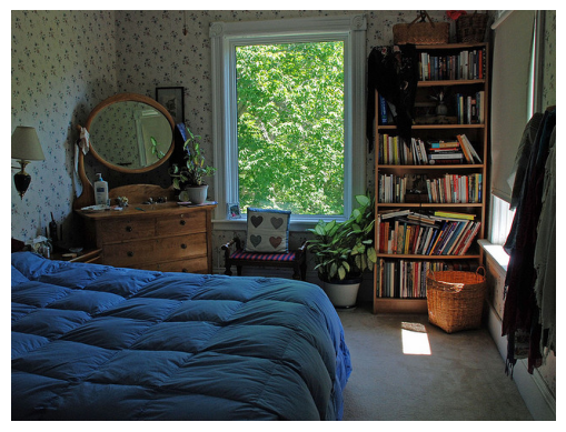
Generated caption: a bedroom with a bed and a windowVisual Question Answering (VQA) is a task that generates answers to questions about an image based on its content. If image captioning describes the content of an image, VQA is a question-answering process for images. For example, it answers questions like “What is the cat eating?” VQA requires more complex and high-dimensional image understanding capabilities than image captioning, especially the ability to understand and infer the relationship between the image and the question (text).
Like image captioning, early VQA models used a structure that combined CNN and RNN. They extracted image features using CNN, encoded questions using RNN, and then combined these two features to generate answers. However, simply combining image features and question features made it difficult to answer complex questions.
As the attention mechanism was successful in image captioning, it was also introduced to VQA. Co-Attention applies attention to both images and questions, calculating the relevance between each word of the question and each region of the image. This allows for more accurate identification of image regions related to the question.
Stacked Attention repeats attention multiple times to gradually understand the complex relationship between the image and the question. It’s similar to a detective looking at a picture multiple times to deeply understand its relevance to the question.
Representative models include Stacked Attention Networks (SAN) (Yang et al., 2016) and Dual Attention Networks (DAN) (Nam et al., 2017). SAN is a model that applies attention to images multiple times to generate answers to questions, while DAN calculates attention separately for images and questions and combines them to generate answers.
The biggest difference between image captioning and VQA is the integration of external knowledge. To further improve the inference capabilities of VQA models, research has been conducted to utilize external knowledge (common sense, encyclopedia knowledge, etc.). The Knowledge Base (KB) uses structured knowledge bases such as Wikipedia and ConceptNet to provide information needed to find answers to questions.
Memory Networks store external knowledge in memory form and use it to generate answers by searching for relevant information in memory according to the question. However, effectively utilizing external knowledge is still a challenging task. There are many problems to be solved, including the imperfection of the knowledge base, judgment of relevance to questions, and complexity of the inference process.
VQA research has added important genes to deep learning DNA. The combination of CNN-RNN shares a basic framework with image captioning for combining images and text. Multimodal attention gives deep learning models the ability to model complex relationships between images and questions. This means that deep learning models can understand and infer interactions between information, rather than just combining it.
External knowledge integration has opened up the possibility for deep learning models to perform higher-level inferences using external knowledge. This shows that deep learning models can utilize human knowledge and experience, rather than just relying on data. 10.2.1 and 10.2.2 sections reviewed image captioning and VQA, which were two important pillars of early multimodal deep learning research. These studies greatly contributed to applying and advancing the core technologies of deep learning, such as CNN, RNN, and attention mechanisms, to multimodal problems, and became an important foundation for the emergence of more powerful multimodal models based on transformers (CLIP, DALL-E, GPT-4V, Gemini, etc.).
Recently, transformer-based VQA models like ViLT (Vision-and-Language Transformer) have emerged, showing good performance. ViLT inputs image patches and text tokens into the same transformer model, effectively modeling complex interactions between images and text.
ViLT (Vision-and-Language Transformer) is one of the representative transformer-based VQA models. ViLT inputs image patches and text tokens into the same transformer model, effectively modeling complex interactions between images and text.
The following is an example code for performing VQA using the ViLT model with the Hugging Face Transformers library.
from transformers import ViltProcessor, ViltForQuestionAnswering
from PIL import Image
import requests
import matplotlib.pyplot as plt

# 모델과 프로세서 로드
processor = ViltProcessor.from_pretrained("dandelin/vilt-b32-finetuned-vqa")
model = ViltForQuestionAnswering.from_pretrained("dandelin/vilt-b32-finetuned-vqa")

# 이미지 다운로드
url = "http://images.cocodataset.org/val2017/000000039769.jpg"
image = Image.open(requests.get(url, stream=True).raw)

# 이미지 출력
plt.imshow(image)
plt.axis('off')  # 축 제거
plt.show()


# 질문 설정
question = "How many cats are in the image?"
print("Question:", question)


# 입력 전처리
encoding = processor(image, question, return_tensors="pt")

# 추론
outputs = model(**encoding)
logits = outputs.logits
idx = logits.argmax(-1).item()
print("Predicted answer:", model.config.id2label[idx])
Question: How many cats are in the image?
Predicted answer: 2Let’s say we have two types of information: images and text. How can we combine these two pieces of information? The simplest way is to concatenate the image vector with the text vector to create a new vector. Connecting information from heterogeneous data sources is called fusion. Efficiently fusing information from two heterogeneous data characteristics is the core of multimodal learning. One reason why it’s difficult to start multimodal deep learning is that it’s a rapidly evolving field, making systematic organization lacking.
In this section, we will explain multimodal fusion in three main categories based on the methods presented in Carnegie Mellon University (CMU) Multimodal Machine Learning lectures. Although this classification is not the standard for current multimodal research, it is very useful for understanding various fusion techniques systematically.
Joint Representations is a method of representing multiple modalities of data in a single common vector space. It’s like drawing text and images together on one canvas.
Instead of processing each modality’s data separately, they are fused into one integrated feature vector. This vector contains the information of each modality, allowing the model to learn deep correlations between modalities. One model can process multiple modalities, and the model structure is relatively simple and efficient because it compresses and represents multiple modalities’ information in one vector. However, each modality’s unique characteristics may be diluted or lost during the fusion process. If a particular modality has much more information than other modalities, an information imbalance problem can occur. Fusing data from different modalities into one meaningful vector is a very difficult problem.
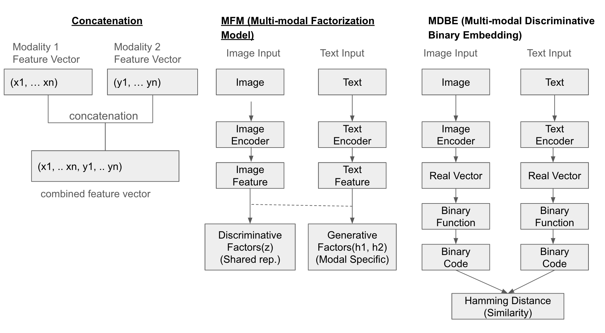
One simple method is to concatenate each modality’s feature vectors. Additionally, the Multi-modal Factorization Model (MFM) combines multiple types of data through matrix factorization to create a common representation space. Multi-modal Discriminative Binary Embedding (MDBE) is a method that represents multimodal data such as images and text as binary codes.
Recent research has proposed methods like COSA (Concatenated Sample), which sequentially connects multiple image-text pairs and applies a transformer-based model to jointly learn visual content and temporal cues. Attentional Concatenation is also used to generate high-resolution images from text, using a multi-level hierarchical structure and utilizing the results of previous layers and word vectors as input for the next layer.
Structural Example
The following diagram illustrates the fusion of three methods (Concatenation, MFM, MDBF).
Example
from transformers import AutoModel, AutoProcessor, AutoTokenizer
from PIL import Image
import torch
import requests
import matplotlib.pyplot as plt

# Load pre-trained models and processor/tokenizer for image and text
image_model_name = "google/vit-base-patch16-224-in21k"  # ViT (Vision Transformer)
text_model_name = "bert-base-uncased"  # BERT

image_processor = AutoProcessor.from_pretrained(image_model_name)
image_model = AutoModel.from_pretrained(image_model_name)
tokenizer = AutoTokenizer.from_pretrained(text_model_name)
text_model = AutoModel.from_pretrained(text_model_name)


# Example image and text
url = "http://images.cocodataset.org/val2017/000000039769.jpg"
image = Image.open(requests.get(url, stream=True).raw)
text = "Two cats sleeping on a couch."

# Display the image
plt.imshow(image)
plt.axis('off')  # Remove axes
plt.show()

# Preprocess image and text
image_inputs = image_processor(images=image, return_tensors="pt")
text_inputs = tokenizer(text, return_tensors="pt")

# Feature extraction (embeddings) for each modality
with torch.no_grad():  # Disable gradient calculation (inference mode)
    image_features = image_model(**image_inputs).last_hidden_state[:, 0, :]  # [CLS] token embedding
    text_features = text_model(**text_inputs).last_hidden_state[:, 0, :]   # [CLS] token embedding


# Create Joint Representation (Concatenation)
joint_representation = torch.cat((image_features, text_features), dim=1)

print("Image Features Shape:", image_features.shape)  # Image feature vector size
print("Text Features Shape:", text_features.shape)     # Text feature vector size
print("Joint Representation Shape:", joint_representation.shape) # Combined feature vector size (image + text)
Fast image processor class <class 'transformers.models.vit.image_processing_vit_fast.ViTImageProcessorFast'> is available for this model. Using slow image processor class. To use the fast image processor class set `use_fast=True`.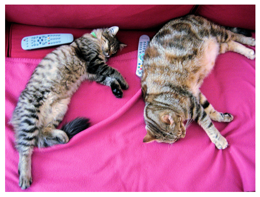
Image Features Shape: torch.Size([1, 768])
Text Features Shape: torch.Size([1, 768])
Joint Representation Shape: torch.Size([1, 1536])Coordinated Representations is a method that represents each modality in a separate space and explicitly learns the relationship between them. It’s similar to having multiple canvas paintings, where each canvas harmonizes with the others.
Each modality is represented as a separate feature vector, but these vectors are learned to “coordinate” with each other. In other words, the feature space of each modality is independent, but their similarities, order relationships, and other meaningful connections are learned to establish a meaningful relationship between them. The advantage of this approach is that it preserves the unique characteristics of each modality while considering its relevance to other modalities. Additionally, it can learn the relationships between various forms of modalities, making it applicable to diverse multi-modal problems.
However, since each modality must be processed separately, the model structure may become more complex than Joint Representations. This can make model design and training more difficult. Furthermore, explicitly learning the relationship between each modality is not an easy task.
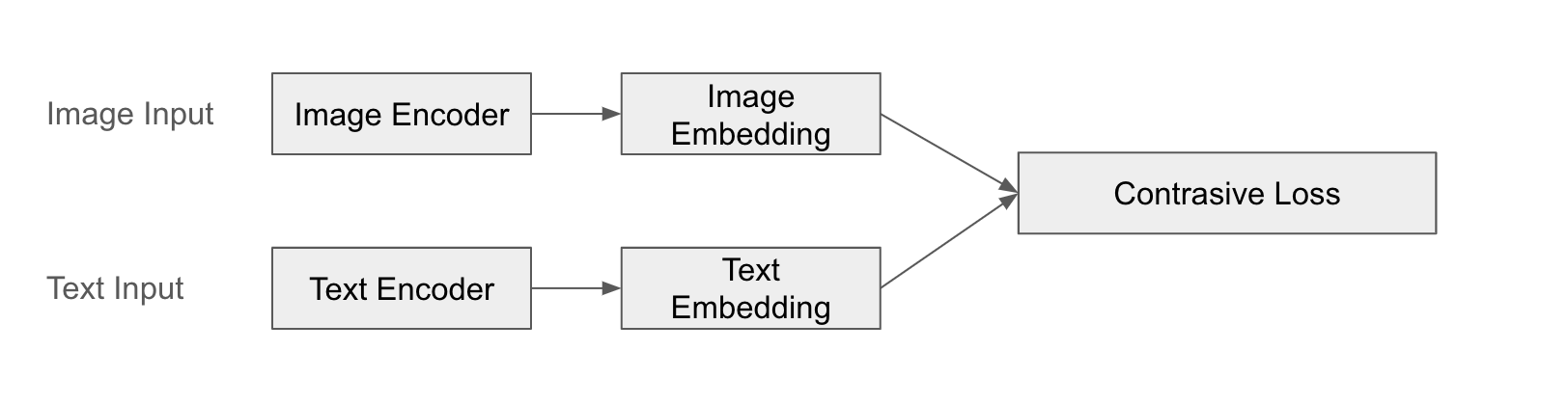
A representative example is CLIP (Contrastive Language-Image Pre-training). CLIP processes images and text through separate encoders to obtain feature vectors and learns their similarity. CLIP learns to pair images and text, allowing it to understand the meaningful relationship between them.
CLIP’s success is particularly notable in its zero-shot learning ability. A pre-trained CLIP model can classify or search for new images without additional training for a specific task. This is possible because it effectively learns the semantic connection between text and images.
Structure Example
The following is a diagram of CLIP’s fusion.
Example
from transformers import CLIPProcessor, CLIPModel
from PIL import Image
import torch
import requests
import matplotlib.pyplot as plt

# Load CLIP model and processor
model = CLIPModel.from_pretrained("openai/clip-vit-base-patch32")
processor = CLIPProcessor.from_pretrained("openai/clip-vit-base-patch32")

# Example image and text
url = "http://images.cocodataset.org/val2017/000000039769.jpg"
image = Image.open(requests.get(url, stream=True).raw)
text = "Two cats sleeping on a couch."

# Display image
plt.imshow(image)
plt.axis('off')  # Remove axes
plt.show()

# Preprocess image and text
inputs = processor(text=[text], images=image, return_tensors="pt", padding=True)

# Extract image and text features (embeddings)
with torch.no_grad():
    outputs = model(**inputs)
    image_features = outputs.image_embeds
    text_features = outputs.text_embeds

# Coordinated Representation: Keep features of each modality separate
print("Image Features Shape:", image_features.shape)
print("Text Features Shape:", text_features.shape)

# Calculate similarity between image and text (dot product)
similarity = torch.matmul(image_features, text_features.T)  # Or text_features @ image_features.T
print("Image-Text Similarity:", similarity.item())
Image Features Shape: torch.Size([1, 512])
Text Features Shape: torch.Size([1, 512])
Image-Text Similarity: 0.29803216457366943
By applying the above method, a simple zero-shot test is possible as follows.
# Zero-shot 이미지 분류
#   - 여러 텍스트 후보군을 만들고, 각 텍스트와 이미지 간의 유사도를 계산하여 가장 높은 유사도를 갖는 텍스트를 선택

candidate_texts = ["a photo of a cat", "a photo of a dog", "a photo of a bird"]
inputs = processor(text=candidate_texts, images=image, return_tensors="pt", padding=True)

with torch.no_grad():
    outputs = model(**inputs)
    image_features = outputs.image_embeds
    text_features = outputs.text_embeds
    logits_per_image = outputs.logits_per_image # 유사도 점수

probs = logits_per_image.softmax(dim=1)  #  확률
predicted_class_idx = probs.argmax().item()
predicted_class = candidate_texts[predicted_class_idx]

print("Predicted Class:", predicted_class)
print("Probabilities:", probs)
Predicted Class: a photo of a cat
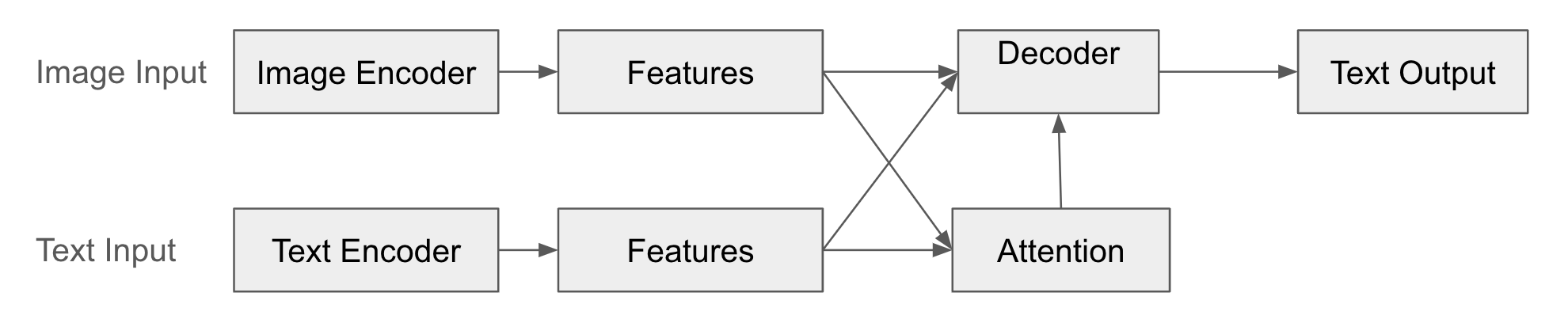
Probabilities: tensor([[9.9403e-01, 5.1377e-03, 8.3070e-04]])The Encoder-Decoder is a method of converting data from one modality to another. It is a technique commonly used in language translation.
In this structure, the encoder converts the input modality data (e.g., image) into a feature vector. This feature vector compactly represents the core information of the input data. The decoder generates data of another modality (e.g., text) based on the feature vector created by the encoder. The decoder “interprets” the output of the encoder to create new data. Additionally, through the attention mechanism, the decoder learns which part of the encoder’s feature vector to “pay attention” to when generating output data.
The advantage of this method is that it can be applied to various tasks that connect different forms of data, such as image captioning, VQA, and machine translation. It can also be applied even if the input and output modalities are different, and various combinations such as text-image, image-text, and audio-text are possible.
Representative examples include image captioning and VQA (Visual Question Answering). Image captioning processes an image with an encoder to obtain a feature vector and uses a decoder to generate a caption (text). VQA processes an image and a question (text) separately with encoders, uses an attention mechanism to understand the relationship between the image and the question, and then uses a decoder to generate an answer (text).
However, if the input or output data becomes longer, information loss may occur or the amount of computation may increase. In particular, in the case of RNN-based models, it may be difficult to learn long-distance dependencies due to the gradient vanishing problem. Additionally, since the encoder and decoder must be trained simultaneously, training can be unstable or difficult.
Structure Example
The following is a diagram of the Encoder-Decoder fusion.
Example
from transformers import BlipProcessor, BlipForConditionalGeneration
from PIL import Image
import requests
import matplotlib.pyplot as plt

# Load model and processor
processor = BlipProcessor.from_pretrained("Salesforce/blip-image-captioning-base")
model = BlipForConditionalGeneration.from_pretrained("Salesforce/blip-image-captioning-base")

# Download image
url = "http://images.cocodataset.org/val2017/000000000139.jpg"
image = Image.open(requests.get(url, stream=True).raw)

# Display image
plt.imshow(image)
plt.axis('off')
plt.show()

# Input text (optional - Conditional Generation)
# text = "describe this image:"  # Prompt (guide image description)
text = "a photo of"

# Preprocess image and text (optional)
# If text is provided, it uses the text as a prompt to generate the caption.
inputs = processor(image, text=text, return_tensors="pt")

# Generate caption
outputs = model.generate(**inputs)

# Decode and print caption
caption = processor.decode(outputs[0], skip_special_tokens=True)
print("Generated caption:", caption)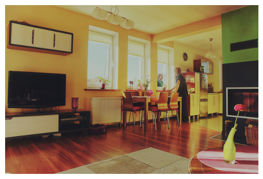
Generated caption: a photo of a living room with a television and a fireplaceThis example shows image captioning, a representative example of the Encoder-Decoder structure. The encoder takes an image (BLIP’s visual encoder) as input and extracts feature vectors. The decoder generates text (BLIP’s text decoder). It determines which part of the image feature vector to focus on through the attention mechanism while generating captions. You can specify a prompt that affects the caption generated as text. Although BLIP can use both images and text as inputs, here we only use images as inputs and generate text in the decoder.
In sections 10.3.1, 10.3.2, and 10.3.3, we looked at the three core theories of multimodal fusion: Joint Representations, Coordinated Representations, and Encoder-Decoder. Each method has its own characteristics and advantages and disadvantages, so it is important to select the appropriate method according to the application field.
In multimodal deep learning, “fusion” refers to the core process of combining information from different modalities to create a richer and more powerful representation. Although we briefly reviewed CMU lecture-based fusion theory in Section 10.3, actual multimodal fusion research has been much more diverse and dynamic. In this deep dive, we will analyze various classification systems for fusion and the latest research trends in depth, and examine which technologies are being noted as of 2025.
Multimodal fusion is difficult to classify based on a single criterion. Researchers classify fusion methods from various perspectives, and each classification is not mutually exclusive but complementary.
This classification focuses on “which stage” of the multimodal deep learning model the fusion occurs. (Refer to Section 10.3.4)
Early Fusion: Combines “raw” data (or features processed very early) from each modality at the input stage of the model.
Late Fusion: Processes each modality with a separate model and combines the outputs (e.g., prediction results) at the final stage.
Hybrid Fusion: Combines Early Fusion and Late Fusion. It performs fusion at multiple stages of the model to utilize information at various levels.
Model-Agnostic Fusion: General fusion techniques that do not depend on specific models (e.g., Early, Late, Hybrid Fusion).
Model-Specific Fusion: Fusion techniques specialized for specific model structures.
Latest Research: The MULA 2025 workshop, to be held on June 11-12, 2025, will discuss model structures for effectively fusing various sensor data (camera, LiDAR, radar, etc.) in the field of autonomous driving. This workshop aims to encourage interdisciplinary interactions and collaborations between computer vision, multimedia, remote sensing, and robotics communities, with a particular focus on multimodal approaches in autonomous driving.
Symmetric vs. Asymmetric Fusion:
Symmetric: Treats all modalities equally.
Asymmetric: Gives more weight to certain modalities or assigns different roles.
Latest Research: “Learning Deep Multimodal Feature Representation with Asymmetric Multi-layer Fusion” proposed an effective framework for fusing multimodal features in multiple layers within a single network. This study introduced two asymmetric fusion operations, channel shuffle and pixel shift, to learn different features according to various fusion directions. Additionally, “Multimodal sentiment analysis based on multi-layer feature fusion,” published in January 2025, presented a new approach for accurate sentiment analysis under modal imbalance and implicit expression conditions.
Explicit vs. Implicit Fusion:
Explicit: Explicitly defines or models the relationships between modalities (e.g., attention mechanisms).
Implicit: Does not directly define the relationships between modalities, but rather allows the model to learn them through training (e.g., simple concatenation).
Latest Research: The HCI International 2025 conference (June 2025) will feature a study comparing the pros and cons of explicit and implicit fusion.
The most notable fusion method in 2024-2025 research is the attention-based mechanism.
Concept: Applies attention to the features of one modality (key-value) using the features of another modality as a query. (Refer to Section 10.4.2) This allows the model to finely capture the relationships between specific elements of different modalities.
Advantages: Can capture fine-grained and flexible relationships between modalities. For example, in image captioning, it can focus on the “running” action of a dog in the image when generating the word “running.”
Latest Research
The “Bi-Att3DDet” study, published in January 2025, introduced a bidirectional attention-based fusion method for 3D object detection in autonomous driving. This study proposed a bidirectional interaction approach to maximize the utilization of complementary information between LiDAR and camera data.
The “LANMSFF” study, published in March 2024 and revised in February 2025, combined a lightweight attention-based network with multi-scale feature fusion for multi-view facial expression recognition. This approach simultaneously generates channel and spatial attention maps to emphasize important features and suppress irrelevant ones.
A recent neuroscience study (2025) investigated the impact of cross-modal congruency on sensory information processing and accumulation. The study showed that congruence between auditory and visual stimuli plays a crucial role in the early stages of sensory processing. #### 2.2 Multi-head Attention
Concept: Uses multiple attention heads to capture relationships between modalities from different perspectives. Each head uses different weight matrices (W_Q, W_K, W_V) to transform the input data and calculate attention, allowing each head to focus on different aspects of the input data (e.g., meaning, grammatical structure, style).
Advantages: Can model various types of relationships simultaneously, enabling the learning of richer and more complex representations. For example, when fusing images and text, some heads can focus on the relationship between objects in the image and words in the text, while others focus on the relationship between the overall atmosphere of the image and the tone of the text.
Recent Research: Recent large-scale multi-modal models (LMMs) have further expanded and refined this technique, effectively modeling complex interactions between various modalities such as images, text, audio, and video.
Contrastive Learning:
Concept: Learns to place related modality pairs (e.g., an image and its caption) close together in the embedding space and unrelated pairs far apart.
Advantages: Can be effectively learned from large-scale unlabeled datasets, helping to alleviate data scarcity issues.
Recent Research: “Dual-Level Cross-Modal Contrastive Clustering” (2024) proposes a new contrastive learning method to bridge the gap between visual representations and text semantics.
Masking-Based Learning:
Concept: Masks parts of the input and learns to recover them using information from other modalities.
Advantages: Can learn complementary relationships between modalities. For example, it can learn to predict masked parts of an image using text descriptions or predict masked words in text using images.
Recent Research: CAST (2025) improved the alignment between graph structure nodes and text tokens through a Masked Node Prediction (MNP) pre-training strategy.
Token-Level Fusion: Models fine-grained interactions between individual tokens of each modality (e.g., image patches, text tokens).
Advantages: Enables more nuanced capture of relationships between modalities. For example, it can learn direct correspondence relationships between specific objects in an image and specific words in text.
Recent Research: CAST (2025) demonstrated that token-level fusion outperforms instance-level fusion in the field of materials science, particularly in graph node and text token fusion.
Instance-Level Fusion: Treats each modality’s entire instance (e.g., an entire image, entire text) as a single unit for fusion.
Advantages: High computational efficiency and simple implementation.
Disadvantages: May fail to capture detailed relationships within modalities.
Multi-modal fusion can be classified in various ways, each providing different perspectives. In actual research, these classifications are often combined and used together. As of 2025, multimodal fusion research focuses on developing efficient fusion techniques using fine-grained interactions at the token level, cross-attention mechanisms, and self-supervised learning methods. In particular, major academic events such as the CVPR 2025 workshop (June 2025, Nashville) will actively discuss advances in multimodal fusion technology in various application fields, including autonomous driving, medical diagnosis, and materials science.
Through this deep dive, we will understand the various classification systems of multimodal fusion and grasp the characteristics of each approach, allowing us to analyze the various multimodal models introduced later more in-depth.
There is no original text provided to translate.
From Sections 10.3.1 to 10.3.3, we examined ways to fuse multimodal data. This is a theoretical classification. When actually designing a multimodal model, it is necessary to strategically decide which fusion method to apply, when, and how, according to the characteristics of the given problem and data. In this section, we will look at sophisticated modality integration strategies adopted by state-of-the-art multimodal models.
Early fusion combines the inputs of multiple modalities in the early stages of the model. The simplest form is to concatenate the feature vectors of each modality. The advantage of early fusion is that it is easy to capture low-level interactions between modalities. For example, if the color of an image and a specific word in text are strongly related, early fusion can easily learn this relationship. However, it may not fully utilize the characteristics of each modality. In particular, when specialized processing is required for each modality (e.g., CNN for images and RNN for text), early fusion can be inefficient.
Recent studies have also presented benchmarks that validate the effectiveness of early fusion in environments with noisy multimodal data, beyond simple concatenation.
Let’s take a look at a simple example of early fusion. This is an example where joint representation uses concatenation for early fusion. The same code is used. Finally, a simple linear classifier is used to determine whether there is a cat or not.
from transformers import AutoModel, AutoProcessor, AutoTokenizer
from PIL import Image
import torch
import requests
import matplotlib.pyplot as plt

# 이미지와 텍스트를 위한 사전 학습된 모델 및 프로세서/토크나이저 로드
image_model_name = "google/vit-base-patch16-224-in21k"  #  ViT (Vision Transformer)
text_model_name = "bert-base-uncased"  # BERT

image_processor = AutoProcessor.from_pretrained(image_model_name)
image_model = AutoModel.from_pretrained(image_model_name)
tokenizer = AutoTokenizer.from_pretrained(text_model_name)
text_model = AutoModel.from_pretrained(text_model_name)


# 예제 이미지 및 텍스트
url = "http://images.cocodataset.org/val2017/000000039769.jpg"
image = Image.open(requests.get(url, stream=True).raw)
text = "Two cats sleeping on a couch."

# 이미지 출력
plt.imshow(image)
plt.axis('off')  # 축 제거
plt.show()


# 이미지와 텍스트 전처리
image_inputs = image_processor(images=image, return_tensors="pt")
text_inputs = tokenizer(text, return_tensors="pt")

# 각 모달리티에 대한 특징 추출 (임베딩)
with torch.no_grad():  # 기울기 계산 비활성화 (추론 모드)
    image_features = image_model(**image_inputs).last_hidden_state[:, 0, :]  # [CLS] 토큰 임베딩
    text_features = text_model(**text_inputs).last_hidden_state[:, 0, :]   # [CLS] 토큰 임베딩


# Joint Representation 생성 (Concatenation)
joint_representation = torch.cat((image_features, text_features), dim=1)

print("Image Features Shape:", image_features.shape)  # 이미지 특징 벡터 크기
print("Text Features Shape:", text_features.shape)     # 텍스트 특징 벡터 크기
print("Joint Representation Shape:", joint_representation.shape) # 결합된 특징 벡터 크기 (image + text)

#  Joint Representation을 활용한 추가 작업 (예: 분류)
num_labels = 2  #  예: "고양이 없음(0)" "고양이 있음(1)", 두 가지 클래스로 분류
classifier = torch.nn.Linear(joint_representation.size(1), num_labels) # 간단한 선형 분류기
outputs = classifier(joint_representation)
print("Classification Outputs:", outputs)
Fast image processor class <class 'transformers.models.vit.image_processing_vit_fast.ViTImageProcessorFast'> is available for this model. Using slow image processor class. To use the fast image processor class set `use_fast=True`.
Image Features Shape: torch.Size([1, 768])
Text Features Shape: torch.Size([1, 768])
Joint Representation Shape: torch.Size([1, 1536])
Classification Outputs: tensor([[0.1817, 0.0355]], grad_fn=<AddmmBackward0>)
In the above example, the image and text are directly combined as the output of separate models, ViT and BERT. No additional processing (attention, complex transformation, etc.) is performed on these two vectors before combining the image features and text features. Therefore, this corresponds to early fusion.
Late fusion processes each modality with a separate model and combines the outputs of each model (e.g., prediction results) in the final stage. The advantage of this approach is that it can use models specialized for each modality. For example, pre-trained CNN can be used for images and pre-trained Transformer can be used for text to effectively extract complex features from each modality. However, it only considers high-level interactions between modalities and has a disadvantage that information exchange in the middle stage is difficult.
Late fusion is similar to ensemble techniques, and there are active studies on combining the outputs of models for different modalities to improve performance.
Hybrid fusion combines early fusion and late fusion. It performs fusion at multiple stages of the model to utilize various levels of information. The advantage of this approach is that it can take advantage of both early fusion and late fusion. In other words, it can consider both low-level and high-level interactions between modalities. However, the model structure becomes complex, and there are many hyperparameters to tune.
A representative example of hybrid fusion is Cross-Modal Attention. This method uses the features of one modality as a query to apply attention to the features (key-value) of another modality. This is a representative method for performing fusion in the middle stage.
Recently, in addition to attention, various methods such as gated mechanisms and bilinear pooling have been attempted for mid-level fusion.
Since 2023, large-scale multi-modal models (LMMs) such as Gemini and GPT-4V have introduced more refined modality integration strategies to greatly improve performance.
Selective Fusion Mechanism dynamically determines the importance of each modality and selectively integrates information. For example, when text is included in an image, it strongly associates the visual features of the text area with the text content. This is similar to how humans adjust the importance of visual and textual information according to the situation.
Dynamic Weighting automatically adjusts the contribution of each modality based on the characteristics of the task and input. For example, in visual question answering (VQA) tasks, it assigns different weights to image and text information depending on the nature of the question. For a question like “What is the color of the image?”, it gives more weight to visual information, while for a question like “What does the image mean?”, it gives more weight to textual information.
Task-Specific Fusion optimizes the modality integration method according to the requirements of a specific task. In image captioning, it focuses on one-way transfer from visual to text information, while in visual question answering, it enhances two-way interaction.
These refined integration strategies have greatly improved the performance of multi-modal models. In particular, by dynamically adjusting the role and importance of each modality and optimizing the fusion method according to the task characteristics, they have shown excellent results in tasks that require complex inference, beyond simple information combination. These integrated strategies require large datasets and computational resources, so it is difficult to implement and experiment directly through learning examples. Instead, it is desirable to understand conceptually through the papers and technical documents of each model.
In Section 10.3, we examined various theoretical methods and strategies for fusing multimodal data. Based on this, let’s take a look at the specific techniques that actual multimodal models use to effectively represent information from each modality and learn relationships between different modalities. The entire implementation is in chapter_10/multimodal_embeding.py.
One of the core tasks in multimodal learning is how to represent modalities with different characteristics in a meaningful common space. Images are 2D arrays of pixel values, text is a 1D sequence of tokens, and audio is amplitude values over time, each with its own unique representation method. To effectively process these heterogeneous data, a representation learning technique is needed that captures the essential characteristics of each modality while maintaining the semantic relationships between them.
Early Approach: Individual Encoders + Projection
Early multimodal models used specialized encoders for each modality (e.g., CNN for images, RNN for text) to extract feature vectors, which were then projected into a common vector space using linear transformation or shallow MLP. (Refer to Joint Representation and Concatenation methods in Section 10.3.1)
Recent Approach: Semantic Alignment
Recently, the main approach is to learn semantic alignment between modality-specific feature vectors, rather than simply matching dimensions. In other words, related images and text are learned to be close in the embedding space, while unrelated images and text are learned to be far apart.
Contrastive Learning: (Refer to Coordinated Representation and CLIP example in Section 10.3.2) Image-text pairs are considered “positive” samples, and randomly mixed image-text pairs are considered “negative” samples. The model learns to increase the similarity between positive samples and decrease the similarity between negative samples.
Triplet Loss: Using an image anchor, a positive text (the caption of the anchor image), and a negative text (the caption of another image), the model learns to make the distance between the anchor image and the positive text close, and the distance between the anchor image and the negative text far.
Implementation Example (Contrastive Learning)
class MultimodalEmbedding(nn.Module):
    def __init__(self, embedding_dim=512):
        super().__init__()
        self.image_encoder = models.resnet18(pretrained=True)
        self.image_encoder.fc = nn.Sequential(
            nn.Linear(512, embedding_dim),
            nn.LayerNorm(embedding_dim)
        )

        self.text_encoder = BertModel.from_pretrained('bert-base-uncased')
        self.text_projection = nn.Sequential(
            nn.Linear(768, embedding_dim),  # BERT output dimension is 768
            nn.LayerNorm(embedding_dim)
        )

        self.logit_scale = nn.Parameter(torch.ones([]) * np.log(1 / 0.07))

    def encode_image(self, image):
        return self.image_encoder(image)

    def encode_text(self, input_ids, attention_mask):
        text_features = self.text_encoder(input_ids, attention_mask)[0][:, 0, :]  # [CLS] token, keep batch dim
        return self.text_projection(text_features)
MultimodalEmbedding class:
image_encoder: Uses ResNet18 to convert an image into a feature vector of size embedding_dim.text_encoder: Employs the BERT model to convert text into a feature vector and aligns it to the size of embedding_dim through the text_projection layer.logit_scale: A learnable temperature parameter used in CLIP.Semantic Alignment Mechanism
The semantic alignment is largely implemented in two parts: the forward method of the MultimodalEmbedding class and the constrasive_loss().
def forward(self, image, input_ids, attention_mask):
    image_features = self.encode_image(image)
    text_features = self.encode_text(input_ids, attention_mask)

    image_features = image_features / image_features.norm(dim=-1, keepdim=True)
    text_features = text_features / text_features.norm(dim=-1, keepdim=True)

    logit_scale = self.logit_scale.exp()
    logits = logit_scale * image_features @ text_features.transpose(-1, -2)
    # print("logits:", logits.shape)

    return logits   # Return a single value
forward method:
Uses encode_image and encode_text to encode the image and text, respectively.
Feature Normalization: Applies L2 normalization to set the magnitude of image_features and text_features vectors to 1. This is done to consider only the direction of the vectors when calculating similarity.
Temperature Scaling: Utilizes logit_scale to adjust the distribution of similarity scores. The logit scale is applied to an exponential function to obtain a scaling value, which is then multiplied with the matrix product of the image feature matrix and the transposed text feature matrix. The matrix product calculates the dot product between each image feature vector and all text feature vectors to generate similarity scores.
logits: Calculates the similarity (dot product) between image feature vectors and text feature vectors. Instead of using text_features.t(), text_features.transpose(-1, -2) is used for transposition. This swaps the last two dimensions of the text feature matrix from (batch, text feature dimension) to (batch, feature dimension, text), allowing multiplication with the image feature matrix of shape (batch, image feature dimension).
def contrastive_loss(logits): # removed enhanced_similarity
    labels = torch.arange(logits.size(0), device=logits.device) # Use logits.size(0)

    # Image-to-text and text-to-image contrastive loss
    img_txt_loss = nn.CrossEntropyLoss()(logits, labels)
    txt_img_loss = nn.CrossEntropyLoss()(logits.T, labels)

    # Average loss
    return (img_txt_loss + txt_img_loss) / 2
In the contrastive_loss function, labels are generated as integers from 0 to (batch size - 1) to match the size of the logits matrix. The diagonal elements (i, i) in the logits matrix represent the similarity between the i-th image and the i-th text, which is the similarity of the positive pair (image-text pair), so the labels are set to make these diagonal elements correct. Additionally, img_txt_loss calculates the loss of image-to-text similarity, and txt_img_loss calculates the loss of text-to-image similarity. By averaging these two losses, both image-to-text and text-to-image semantic alignments are considered.
The semantic alignment mechanism maps features from different modalities to a semantically consistent space. First, all feature vectors are projected onto a unit sphere using L2 normalization to remove scale differences between modalities. A temperature scaling parameter is introduced to adjust the distribution of similarity values. High temperatures produce softer distributions, while low temperatures produce sharper distributions, increasing learning stability. Additionally, through contrastive learning, related image-text pairs are learned to be close in the embedding space, and unrelated pairs are learned to be far apart. In particular, both image-to-text and text-to-image mappings are simultaneously optimized to achieve bidirectional semantic alignment.
Like CLIP’s contrastive learning, related content is learned to be close, and unrelated content is learned to be far apart. This contrastive learning-based semantic alignment strategy has evolved from OpenAI’s CLIP in 2021 to Google’s PaLM-E, Anthropic’s Claude, and DeepMind’s Gemini. While early CLIP focused on simple contrastive learning of image-text pairs, newer models capture more nuanced relationships between multiple modalities. In particular, Gemini learns semantic alignments between various modalities such as images, text, audio, and video simultaneously, preserving the unique characteristics of each modality while building an integrated semantic space.
Example Execution
The data used for training is Flicker8k. The EnhancedMultimodalEmbedding (or EnhancedMultimodalEmbedding_no_p) model can be trained on the Flickr8k dataset using the train_multimodal_embedding function. In the main function, the model, data loader, optimizer, etc. are set up, and calling the train_multimodal_embedding function starts the training.
# download flickr8k.
!mkdir data;cd data;wget "https://github.com/awsaf49/flickr-dataset/releases/download/v1.0/flickr8k.zip";unzip -q flickr8k.zip -d ./flickr8k
mkdir: cannot create directory ‘data’: File exists
--2025-03-09 16:33:12-- https://github.com/awsaf49/flickr-dataset/releases/download/v1.0/flickr8k.zip
Resolving github.com (github.com)... 20.200.245.247
Connecting to github.com (github.com)|20.200.245.247|:443... connected.
HTTP request sent, awaiting response... 302 Found
Location: https://objects.githubusercontent.com/github-production-release-asset-2e65be/753516996/d7c62b13-1e50-40ea-8fae-f34a44b1695f?X-Amz-Algorithm=AWS4-HMAC-SHA256&X-Amz-Credential=releaseassetproduction%2F20250309%2Fus-east-1%2Fs3%2Faws4_request&X-Amz-Date=20250309T073156Z&X-Amz-Expires=300&X-Amz-Signature=ff62cf7df8ac3deba8bd6f4f775e164abf03c6d2d6d86d740e5407e52702c6a3&X-Amz-SignedHeaders=host&response-content-disposition=attachment%3B%20filename%3Dflickr8k.zip&response-content-type=application%2Foctet-stream [following]
--2025-03-09 16:33:12-- https://objects.githubusercontent.com/github-production-release-asset-2e65be/753516996/d7c62b13-1e50-40ea-8fae-f34a44b1695f?X-Amz-Algorithm=AWS4-HMAC-SHA256&X-Amz-Credential=releaseassetproduction%2F20250309%2Fus-east-1%2Fs3%2Faws4_request&X-Amz-Date=20250309T073156Z&X-Amz-Expires=300&X-Amz-Signature=ff62cf7df8ac3deba8bd6f4f775e164abf03c6d2d6d86d740e5407e52702c6a3&X-Amz-SignedHeaders=host&response-content-disposition=attachment%3B%20filename%3Dflickr8k.zip&response-content-type=application%2Foctet-stream
Resolving objects.githubusercontent.com (objects.githubusercontent.com)... 185.199.109.133, 185.199.111.133, 185.199.110.133, ...
Connecting to objects.githubusercontent.com (objects.githubusercontent.com)|185.199.109.133|:443... connected.
HTTP request sent, awaiting response... 200 OK
Length: 1112971163 (1.0G) [application/octet-stream]
Saving to: ‘flickr8k.zip’
flickr8k.zip 100%[===================>] 1.04G 56.8MB/s in 19s
2025-03-09 16:33:32 (56.9 MB/s) - ‘flickr8k.zip’ saved [1112971163/1112971163]
import torch
from torchvision import models, transforms
from torch.utils.data import Dataset, DataLoader
# Assuming dldna.chapter_10.multimodal_embedding is in the same directory or Python path.
# Adjust if necessary (e.g., from multimodal_embedding import ...).
from dldna.chapter_10.multimodal_embedding import Flickr8kDataset, MultimodalEmbedding, train_multimodal_embedding, generate_example

# Data transformation setup
transform = transforms.Compose([
    transforms.Resize((224, 224)),
    transforms.ToTensor(),
    transforms.Normalize(mean=[0.485, 0.456, 0.406], std=[0.229, 0.224, 0.225])
])

# Dataset and DataLoader setup
image_dir = './data/flickr8k/Images'  # Replace with the actual path to your image directory
caption_file = './data/flickr8k/captions.txt'  # Replace with the actual path to your caption file
dataset = Flickr8kDataset(image_dir, caption_file, transform=transform)

train_size = int(0.8 * len(dataset))
val_size = len(dataset) - train_size
train_dataset, val_dataset = torch.utils.data.random_split(dataset, [train_size, val_size])

train_loader = DataLoader(train_dataset, batch_size=32, shuffle=True, num_workers=4)
val_loader = DataLoader(val_dataset, batch_size=32, shuffle=False, num_workers=4)

# Model initialization
model = MultimodalEmbedding()

# Model training
train_multimodal_embedding(model, train_loader, val_loader, num_epochs=3)

# Model saving
torch.save(model.state_dict(), 'multimodal_embedding_model.pth')

# Example generation
model_path = 'multimodal_embedding_model.pth'
generate_example(model_path, image_dir, caption_file)
Epoch 1/3: 15%|█▍ | 147/1012 [00:16<01:36, 8.96it/s]Image file not found: ./data/flickr8k/Images/imageEpoch 1/3: 100%|██████████| 1012/1012 [01:53<00:00, 8.90it/s]Epoch 1/3 - Train Loss: 0.9618Epoch 1/3 - Validation Loss: 0.5212
Epoch 1: Saved best model with Validation Loss = 0.5212Epoch 2/3: 52%|█████▏ | 525/1012 [00:59<00:55, 8.84it/s]Image file not found: ./data/flickr8k/Images/imageEpoch 2/3: 100%|██████████| 1012/1012 [01:54<00:00, 8.83it/s]Epoch 2/3 - Train Loss: 0.3393Epoch 2/3 - Validation Loss: 0.4240
Epoch 2: Saved best model with Validation Loss = 0.4240Epoch 3/3: 34%|███▍ | 347/1012 [00:39<01:15, 8.85it/s]Image file not found: ./data/flickr8k/Images/imageEpoch 3/3: 100%|██████████| 1012/1012 [01:54<00:00, 8.83it/s]Epoch 3/3 - Train Loss: 0.2313Epoch 3/3 - Validation Loss: 0.3891
Epoch 3: Saved best model with Validation Loss = 0.3891
Image 0: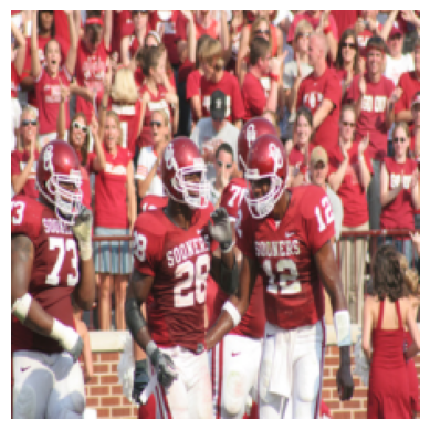
Top 3 Captions (Image -> Text):
  - football players in red congratulate each other as crowds in red cheer behind. (prob: 0.9970)
  - a man in black holds up an obama 08 sign. (prob: 0.0023)
  - a large group of bicycles racing on the street (prob: 0.0004)

Caption: football players in red congratulate each other as crowds in red cheer behind.

Top 3 Images (Text -> Image):
 - Image 0 (prob: 0.9983)
- Image 17 (prob: 0.0013)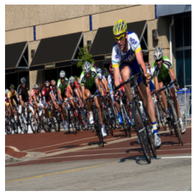
- Image 2 (prob: 0.0001)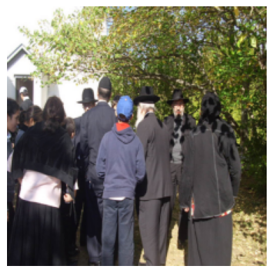
Cross-modal attention is used to effectively model the relationship between different modalities. This extends ViT’s self-attention to enable interaction between heterogeneous data such as images and text.
Modal Attention Design
Cross-modal attention has an asymmetric structure considering the characteristics of each modality.
class CrossModalAttention(nn.Module):
    def __init__(self, config):
        super().__init__()
        self.image_proj = nn.Linear(config.image_dim, config.hidden_dim)
        self.text_proj = nn.Linear(config.text_dim, config.hidden_dim)
        self.attention = nn.MultiheadAttention(config.hidden_dim, config.num_heads)

    def forward(self, image_features, text_features):
        image_proj = self.image_proj(image_features)
        text_proj = self.text_proj(text_features)
        attn_output, _ = self.attention(text_proj, image_proj, image_proj)
        return attn_output
After projecting image and text features into a common latent space, the relationship between the two modalities is learned through a multi-head attention mechanism. The text feature is used as a query, and the image feature is used as a key and value, allowing the text to pay attention to the relevant part of the image.
Asymmetric Attention Pattern
An asymmetric attention pattern is used to preserve the unique characteristics of each modality while facilitating effective information exchange.
class HierarchicalCrossModalAttention(nn.Module):
    def __init__(self, config):
        super().__init__()
        self.local_image_attention = nn.MultiheadAttention(config.hidden_dim, config.num_heads)
        self.local_text_attention = nn.MultiheadAttention(config.hidden_dim, config.num_heads)
        self.image_to_text_attention = CrossModalAttention(config)
        self.text_to_image_attention = CrossModalAttention(config)
        self.output_layer = nn.Linear(config.hidden_dim * 2, config.hidden_dim)

    def forward(self, image_features, text_features):
        local_image = self.local_image_attention(image_features, image_features, image_features)[0]
        local_text = self.local_text_attention(text_features, text_features, text_features)[0]

        image_attended_text = self.image_to_text_attention(image_features, local_text)
        text_attended_image = self.text_to_image_attention(text_features, local_image)

        combined_features = torch.cat([image_attended_text, text_attended_image], dim=-1)
        output = self.output_layer(combined_features)

        return output
Here, bidirectional attention is performed separately from images to text and from text to images. This allows each modality to selectively focus on relevant information from the other modality.
Hierarchical Attention Structure
To capture complex multimodal relationships, multiple layers of attention are hierarchically constructed. In the lower layers, local features within each modality are processed, and in the upper layers, global relationships between modalities are modeled. This hierarchical structure plays a key role in models such as GPT-4V and Gemini.
class EnhancedMultimodalEmbedding_no_p(MultimodalEmbedding):

    def forward(self, image, input_ids, attention_mask):
        image_features = self.encode_image(image)
        text_features = self.encode_text(input_ids, attention_mask)

        image_features = self.image_preserve(image_features)
        text_features = self.text_preserve(text_features)

        combined_features = self.cross_modal_attention(image_features, text_features)

        combined_features = combined_features / combined_features.norm(dim=-1, keepdim=True)

        logit_scale = self.logit_scale.exp()
        logits = logit_scale * combined_features @ combined_features.t()

return logitsimport torch
from torchvision import models, transforms
from torch.utils.data import Dataset, DataLoader
from collections import namedtuple
from dldna.chapter_10.crossmodal_attention import Flickr8kDataset, CrossModalEmbedding, train_crossmodal_embedding, generate_example
# Configuration
config = namedtuple('Config', ['embedding_dim', 'image_dim', 'text_dim', 'hidden_dim', 'num_heads'])(
embedding_dim=512, # Output embedding dimension
image_dim=512, # ResNet18 image encoder output dimension
text_dim=512, # Text feature (768 from BERT -> 512 after projection)
hidden_dim=512, # Cross-modal attention internal hidden dimension
num_heads=8 # Number of multi-head attention heads
)
# Data transformation setup
transform = transforms.Compose([
transforms.Resize((224, 224)),
transforms.ToTensor(),
transforms.Normalize(mean=[0.485, 0.456, 0.406], std=[0.229, 0.224, 0.225])
])
# Dataset and DataLoader setup
image_dir = './data/flickr8k/Images' # Change to the actual path
caption_file = './data/flickr8k/captions.txt' # Change to the actual path
dataset = Flickr8kDataset(image_dir, caption_file, transform=transform)
train_size = int(0.8 * len(dataset))
val_size = len(dataset) - train_size
train_dataset, val_dataset = torch.utils.data.random_split(dataset, [train_size, val_size])
train_loader = DataLoader(train_dataset, batch_size=32, shuffle=True, num_workers=4, pin_memory=True)
val_loader = DataLoader(val_dataset, batch_size=32, shuffle=False, num_workers=4, pin_memory=True)
# Model initialization
model = CrossModalEmbedding(config)
# Model training
train_crossmodal_embedding(model, train_loader, val_loader, num_epochs=3)
# Model saving
torch.save(model.state_dict(), 'crossmodal_embedding_model.pth')Epoch 1/3: 4%|▍ | 40/1012 [00:04<01:41, 9.53it/s]Image file not found: ./data/flickr8k/Images/imageEpoch 1/3: 100%|██████████| 1012/1012 [01:47<00:00, 9.41it/s]Epoch 1/3 - Train Loss: 0.9663Epoch 1/3 - Validation Loss: 0.5378Epoch 2/3: 58%|█████▊ | 582/1012 [01:02<00:45, 9.36it/s]Image file not found: ./data/flickr8k/Images/imageEpoch 2/3: 100%|██████████| 1012/1012 [01:48<00:00, 9.31it/s]Epoch 2/3 - Train Loss: 0.3381Epoch 2/3 - Validation Loss: 0.4452Epoch 3/3: 0%| | 4/1012 [00:00<02:27, 6.82it/s]Image file not found: ./data/flickr8k/Images/imageEpoch 3/3: 100%|██████████| 1012/1012 [01:48<00:00, 9.35it/s]Epoch 3/3 - Train Loss: 0.2288Epoch 3/3 - Validation Loss: 0.3743# Example generation
model_path = 'crossmodal_embedding_model.pth'
generate_example(model_path, image_dir, caption_file)Image 0: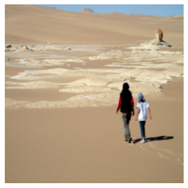
Top 3 Captions (Image -> Text):
  - two people walk out onto the desert sand. (prob: 0.9862)
  - a man takes a picture of him and his friend with his phone. (prob: 0.0092)
  - the little boy wearing the blue shirt is putting dirt in his mouth. (prob: 0.0013)

Caption: two people walk out onto the desert sand.

Top 3 Images (Text -> Image):
 - Image 0 (prob: 0.9898)
- Image 2 (prob: 0.0089)
- Image 4 (prob: 0.0005)
Perceiver is a multimodal architecture proposed by DeepMind in 2021. It addresses the quadratic complexity issue of existing transformers (where computation increases with the square of the input sequence length) while effectively handling various modalities (such as images, text, audio, and point clouds). The Perceiver is particularly advantageous when the input data size is very large (e.g., high-resolution images, long texts). Here, we describe the overall architecture and omit examples. The code is example code for explanation purposes.
Core Idea of Perceiver
Perceiver is based on the following ideas:
Perceiver uses a fixed-size latent array regardless of the input sequence length. This latent array compresses and represents the information of the input data, summarizing a large amount of input information into a small number of latent vectors, like a bottleneck. Therefore, even if the input data size is very large (e.g., 10,000 tokens), the number of latent vectors is fixed (e.g., 256), which can greatly reduce computational complexity and memory usage.
class Perceiver(nn.Module):
    def __init__(self, ..., num_latents=256, latent_dim=512, ...):
        super().__init__()
        # Latent vector initialization (key!)
        self.latents = nn.Parameter(torch.randn(num_latents, latent_dim))
        # ...
In the above code, self.latents represents that latent vector. It is defined as nn.Parameter, which means it is a learnable parameter.
The Perceiver does not use modality-specific processing methods (e.g., CNN, RNN) for input modalities such as images, text, and audio. Instead, each modality undergoes simple preprocessing (e.g., image patches, text tokenization) to be converted into a common format (sequence of vectors). Subsequent processing uses the same transformer-based architecture (Cross-Attention, Self-Attention) regardless of the modality type. This allows for flexible handling of various modalities and easy addition of new modalities.
The Perceiver uses multiple layers of self-attention to gradually update the latent vectors. At each layer, the latent vectors exchange information with each other and learn complex patterns from the input data. Initially, the latent vectors that represented simple features come to express abstract and high-level meanings as they pass through multiple layers.
How Perceiver Works (Simplified Code Example)
import torch
import torch.nn as nn

class Perceiver(nn.Module):
    def __init__(self,
                 input_channels=3,  # Input channels (e.g., RGB image)
                 input_axis=2,      # Input dimension (image=2, video=3)
                 num_latents=256,  # Number of latent vectors
                 latent_dim=512,    # Latent vector dimension
                 num_heads=8,       # Number of attention heads
                 depth=6):          # Model depth (number of self-attention layers)
        super().__init__()

        # 1. Latent vector initialization (key!)
        self.latents = nn.Parameter(torch.randn(num_latents, latent_dim))

        # 2. Input projection (matches input dimension to latent dimension)
        self.input_proj = nn.Linear(input_dim, latent_dim)

        # 3. Cross-Attention (learns relationships between input and latent vectors)
        # self.cross_attention = nn.MultiheadAttention(latent_dim, num_heads, batch_first=True)

        # 4. Self-Attention (learns relationships between latent vectors) - repeated multiple times
        self.self_attention_layers = nn.ModuleList([
            nn.MultiheadAttention(latent_dim, num_heads, batch_first=True)
            for _ in range(depth)
        ])


    def forward(self, x):  # x: Input data (image, text, ...)
        batch_size = x.shape[0]

        # 1. Input projection
        x = self.input_proj(x)

        # 2. Latent vector replication (for each item in the batch)
        latents = self.latents.unsqueeze(0).expand(batch_size, -1, -1)  # (B, num_latents, latent_dim)

        # 3. (Optional) Cross-attention (between input and latent vectors)
        # latents, _ = self.cross_attention(latents, x, x)  # query, key, value

        # 4. Self-attention (between latent vectors) - repeated multiple times
        for layer in self.self_attention_layers:
            latents, _ = layer(latents, latents, latents) # query, key, value

        return latents  # Return the processed latent vectors
Advantages and Disadvantages of Perceiver
Perceiver has the efficiency of having a computational complexity that is almost constant regardless of the input size, and provides flexibility to process various modalities in the same way. Additionally, the expandability of Perceiver, which can easily add new modalities, is also an advantage. However, since Perceiver is still based on a transformer, it has the disadvantage of having a complex structure, and the model can become very large as the dimension of the latent vector and the number of layers increase. Additionally, in specific tasks such as image classification, its performance may be inferior to models specialized for those tasks, such as CNNs.
Perceiver IO
Perceiver IO, a follow-up study to Perceiver, proposed a method to process not only inputs but also outputs through latent vectors. This allows for flexible handling of various output forms (classification, regression, sequence generation, etc.). Perceiver IO is evaluated as a more general and powerful model than Perceiver.
Here, we start with the basic structure of cross-attention and gradually add mechanisms to compare trainability and performance. Through this process, we aim to understand the issues that arise in multimodal learning and explore practical approaches to address them.
When designing cross-attention mechanisms, it is a common and recommended approach to gradually increase complexity as described in this section and experiment with it. This method, known as an ablation study, effectively identifies the importance of each component mechanism and the key elements contributing to the final model’s performance. Many papers proposing new architectures use this approach. Moreover, discussing not only the final performance but also stability issues during training is crucial from a practical perspective.
Comparative Training Methods
Experiments are conducted using the flickr8k dataset, which was previously explored, with text and image as two inputs to train mutual similarity. The training involves versions of cross-attention with increasing complexity. For each version, a cross-attention mechanism is added one by one, and training is performed for comparison. All trainings use the same hyperparameters. The training epoch is fixed at 5.
Structure of Examples
Examples are composed of the following structure:
chapter_10/mm
├── cat_resized.png
├── cross_attention
│   ├── v0.py
│   ├── v1.py
│   ├── v2.py
│   ├── v3.py
│   .... (continue to exist)
├── train_multimodal.py
└── evaluate_models.py
The cross_attention folder increases the complexity of cross-attention sequentially from v1 to v11. train_mulimodal.py dynamically generates and trains the next version of the model after one training is completed. During training, metrics such as accuracy, contrast loss, and execution time are stored to generate a final comparison table. It is not desirable to determine trainability based on loss values and accuracy. The easiest way to check if the training has been done correctly due to the nature of contrastive learning is to evaluate it with data that did not exist before. The file that evaluates the model in a zero-shot manner is evalute_models.py.
The image being evaluated is as follows.

The evaluation is done by measuring the similarity between the above image and five texts.
test_captions = [
    "A dog playing in the park",
    "A cat sleeping on a couch",
    "Children playing soccer",
    "A sunset over the ocean",
    "A person cooking in the kitchen"
]
If the model training is done correctly, the second caption “A cat sleeping on a couch” should have the highest similarity among the five captions. The above image is something that was not in the training data, which corresponds to a typical zero-shot test.
Cross-attention dynamic allocation
Changing the version of cross_attention is done through dynamic allocation.
from dldna.chapter_10.mm.cross_attention.v0 import CrossAttention as v0
from dldna.chapter_10.mm.cross_attention.v1 import CrossAttention as v1
# ... (import other versions) ...
from dldna.chapter_10.mm.cross_attention.v11 import CrossAttention as v11

def get_cross_attention(version, config=None):
    if config is None:
        config = {}

    if version == 'v0':
        return v0(**config)
    elif version == 'v1':
        return v1(**config)
    # ... (other version conditions) ...
    elif version == 'v11':
        return v11(**config)
    else:
        raise ValueError(f"Invalid cross-attention version: {version}")

# ...

class ImageTextMatchingModel(nn.Module):
    def __init__(self, image_encoder_dim=2048, text_encoder_dim=768, projection_dim=256):
        super().__init__()
        self.image_encoder = ImageEncoder(image_encoder_dim, projection_dim)
        self.text_encoder = TextEncoder(text_encoder_dim, projection_dim)

        # The CrossAttention module is dynamically assigned in main().
        self.cross_attention = None  # CrossAttention(projection_dim)

    def forward(self, image, input_ids, attention_mask):
        # ...
        image_attended, text_attended = self.cross_attention(
            image_features.unsqueeze(1),
            text_features.unsqueeze(1)
        )
        # ...

# ...
def run_training(model_versions, ...):
    # ...
    for model_version in model_versions:
        # ...
        # Model initialization
        model = ImageTextMatchingModel()

        # Dynamically load the CrossAttention module
        model.cross_attention = get_cross_attention(model_version, config=config)
        # ...
This part implements the logic to dynamically load and apply various versions of the Cross-Attention module, which is the core of the experiment. The get_cross_attention function takes a string version (v0, v1, …, v11) as input and returns an instance of the CrossAttention class corresponding to that version. Inside the run_training function, for each version specified in the model_versions list, the ImageTextMatchingModel is initialized, and the get_cross_attention function is called to assign the Cross-Attention module of the corresponding version to model.cross_attention.
This dynamic assignment method increases code reusability and makes experiment management easier. When adding a new version of Cross-Attention, you only need to add that version to the get_cross_attention function, so there is no need to greatly modify the training code. Additionally, it is easy to control which versions to train through the model_versions list in the run_training function.
Contrastive Loss calculation and training loop
def contrastive_loss(logits):
    labels = torch.arange(len(logits), device=logits.device)
    loss_i = nn.CrossEntropyLoss()(logits, labels)
    loss_t = nn.CrossEntropyLoss()(logits.t(), labels)
    return (loss_i + loss_t) / 2

def train(model, train_loader, val_loader, epochs=10, lr=1e-4, model_version='v0'):
    # ...
    for epoch in range(epochs):
        model.train()
        total_loss = 0
        # ...
        for batch in tqdm(train_loader, ...):
            images, input_ids, attention_mask = [x.to(device) for x in batch]

            optimizer.zero_grad()
            logits = model(images, input_ids, attention_mask)
            loss = contrastive_loss(logits)

            loss.backward()
            optimizer.step()

            total_loss += loss.item()
        # ... (validation 및 지표 계산) ...
This part defines the calculation of Contrastive Loss used for model training and the training loop. The contrastive_loss function calculates the Contrastive Loss by taking the similarity score (logits) of image-text pairs as input. At this time, the correct label is generated so that the elements corresponding to the diagonal (i.e., the image-text pair with the same index) of the logits are 1 (similar) and the rest are 0 (not similar) (using torch.arange). Both the image-based Cross-Entropy Loss (loss_i) and the text-based Cross-Entropy Loss (loss_t) are calculated, and their average is used as the final loss.
Training method: adding mechanisms
We will test by adding functions one by one from the simplest attention structure. Let’s call the added functions “mechanisms.” As each mechanism is added, we will look at which mechanism affects the multimodal attention design. First, we will take a look at part of the training code, and then we will look directly at the training results. After that, we will also look at which mechanisms determined the success or failure of the training in each cross-modal attention.
The following is the training code. When trained, each model is saved as model_final_{version}.pth. This saved model is used for evaluation.
from dldna.chapter_10.mm.train_multimodal import run_training

# model_versions = ['v0', 'v1']  # List of model versions to train
model_versions = ['v0', 'v1', 'v2', 'v3', 'v4', 'v5', 'v6', 'v7', 'v8', 'v9', 'v10_1', 'v10_2', 'v10_3', 'v10_4', 'v10_5', 'v10_6', 'v11']
epochs = 5
lr = 1e-4

# Dataset
image_dir = './data/flickr8k/Images'  # Change to the actual path
caption_file = './data/flickr8k/captions.txt'  # Change to the actual path

results_df = run_training(model_versions, epochs=epochs, lr=lr, image_dir=image_dir, caption_file=caption_file) # Train multiple versions

# Print results
print("\nTraining Results:")
# Print results in Markdown table format
print(results_df.to_markdown(index=False))
Evaluate with the model.
from dldna.chapter_10.mm.evaluate_models import evaluate_all_models

# Test captions (fixed)
test_captions = [
    "A dog playing in the park",
    "A cat sleeping on a couch",
    "Children playing soccer",
    "A sunset over the ocean",
    "A person cooking in the kitchen"
]

# Run model evaluation
image_path = './cat_resized.png'
model_dir = '.'
model_versions = ['v0', 'v1', 'v2', 'v3', 'v4', 'v5', 'v6', 'v7', 'v8', 'v9', 'v10_1', 'v10_2', 'v10_3', 'v10_4', 'v10_5', 'v10_6', 'v11']

results_df = evaluate_all_models(model_dir, image_path, test_captions, model_versions)

# Print results (Markdown table)
print(results_df.to_markdown(index=False))

# Print results (detailed)
for _, row in results_df.iterrows():
    print(f"\nModel: {row['model_version']}")
    print(f"  Best Caption: {row['best_caption']}")
    print(f"  Trained Well: {row['trained_well']}")
    print(f"  Similarity Ratio: {row['similarity_ratio']}")
    print(f"  Similarity Gap: {row['similarity_gap']}")
    print("  All Similarities:")
    for caption, sim in zip(test_captions, row['all_similarities']):
print(f" - {caption:<30}: {sim}")| model_version | best_caption | all_similarities | similarity_ratio | similarity_gap | trained_well | similarity_ratio_rank |
|---|---|---|---|---|---|---|
| v0 | A cat sleeping on a couch | [‘5.322’, ‘15.477’, ‘-4.509’, ‘-6.609’, ‘2.107’] | 2.908 | 10.155 | True | 1 |
| v1 | A cat sleeping on a couch | [‘3.117’, ‘18.174’, ‘-6.475’, ‘-1.825’, ‘8.705’] | 2.088 | 9.469 | True | 3 |
| v2 | A cat sleeping on a couch | [‘3.085’, ‘12.541’, ‘-4.252’, ‘0.924’, ‘6.849’] | 1.831 | 5.692 | True | 5 |
| v3 | Children playing soccer | [‘34.882’, ‘34.882’, ‘34.882’, ‘34.882’, ‘34.882’] | 1 | 0 | False | 14 |
| v4 | A cat sleeping on a couch | [‘7.385’, ‘8.301’, ‘-1.038’, ‘-6.262’, ‘1.240’] | 1.124 | 0.915 | True | 12 |
| v5 | Children playing soccer | [‘27.357’, ‘27.357’, ‘27.357’, ‘27.357’, ‘27.357’] | 1 | 0 | False | 14 |
| v6 | A cat sleeping on a couch | [‘5.022’, ‘14.861’, ‘-5.370’, ‘-8.630’, ‘9.063’] | 1.64 | 5.798 | True | 7 |
| v7 | A dog playing in the park | [‘16.300’, ‘16.300’, ‘16.300’, ‘16.300’, ‘16.300’] | 1 | 0 | False | 14 |
| v8 | A cat sleeping on a couch | [‘9.841’, ‘15.442’, ‘-7.350’, ‘-1.249’, ‘11.023’] | 1.401 | 4.419 | True | 10 |
| v9 | A cat sleeping on a couch | [‘10.382’, ‘15.192’, ‘-5.582’, ‘-1.594’, ‘5.953’] | 1.463 | 4.81 | True | 9 |
| v10_1 | A dog playing in the park | [‘0.940’, ‘0.472’, ‘-0.554’, ‘0.334’, ‘-0.111’] | 1.991 | 0.468 | False | 4 |
| v10_2 | A cat sleeping on a couch | [‘17.720’, ‘17.720’, ‘17.720’, ‘17.720’, ‘17.720’] | 1 | 0 | True | 14 |
| v10_3 | A cat sleeping on a couch | [‘0.516’, ‘1.479’, ‘-0.989’, ‘-5.989’, ‘5.151’] | 1.748 | 4.421 | True | 6 |
| v10_4 | A cat sleeping on a couch | [‘5.913’, ‘10.334’, ‘-5.989’, ‘-1.024’, ‘5.151’] | 1.748 | 4.421 | True | 6 |
| v10_5 | A cat sleeping on a couch | [‘6.601’, ‘9.990’, ‘-5.984’, ‘-2.988’, ‘-0.070’] | 1.513 | 3.389 | True | 8 |
| v10_6 | A dog playing in the park | [‘33.967’, ‘33.302’, ‘31.580’, ‘32.710’, ‘31.384’] | 1.02 | 0.665 | False | 13 |
| v11 | A cat sleeping on a couch | [‘11.315’, ‘15.491’, ‘-10.428’, ‘-0.004’, ‘10.014’] | 1.369 | 4.175 | True | 11 |
Based on these experimental results, we can analyze the training outcomes for each cross-attention version and summarize the causes of success/failure as follows.
| Version | Attention Structure | Key Features | Training Result | Detailed Explanation |
|---|---|---|---|---|
| v0 | Independent Bidirectional Attention | Only scaled dot-product attention | Training Success | Most basic structure. Calculates attention independently for images and text. No normalization/transformation other than scaling. Without separate normalization, it’s sensitive to changes in input feature scale. |
| v1 | Shared Attention | Single attention matrix and transpose matrix | Training Success | Shares the same attention matrix for image→text and text→image attention calculations. Attempts bidirectional information exchange but remains sensitive to input scale due to lack of normalization and fails to properly reflect asymmetric relationships between the two modalities. |
| v2 | Shared Attention + LN | LayerNorm applied to inputs | Training Success | Applies LayerNorm to input features to stabilize feature scaling. Resolves v1’s issue (input scale sensitivity). Attention matrix is still shared. |
| v3 | v2 + Residual Connection | Adds residual connection to output | Training Failure | Adds residual connection that directly adds original features (image_features, text_features) after attention calculation. This excessively preserves original features, hindering the creation of new features through interaction between modalities. This phenomenon is particularly pronounced in shallow network structures. |
| v4 | v2 + Projection | Modality-specific linear transformations | Training Success | Applies independent linear projections (self.image_proj, self.text_proj) to each modality. By applying separate linear transformations to normalized inputs (image_norm, text_norm), it more flexibly adjusts each modality’s feature space and transforms it into a form suitable for attention calculation. |
| v5 | v2 + Mixing Ratio | Fixed 0.5 mixing ratio | Training Failure | Mixes original features (image_norm, text_norm) and attention outputs (image_attended, text_attended) at a fixed ratio (0.5). Similar to residual connection (v3) in preserving original features, but the fixed mixing ratio limits the model’s ability to flexibly adjust weights according to data. |
| v6 | Shared Attention + Q/K/V | Q/K/V transformations and single LayerNorm | Training Success | Adds separate linear transformations (self.to_q, self.to_k, self.to_v) that generate Query (Q), Key (K), and Value (V) for inputs (image_norm, text_norm). This allows the attention mechanism to learn richer feature representations. Still uses a shared attention matrix. |
| v7 | Shared Multi-head | Multi-head + output normalization | Training Failure | Extends shared attention matrix to multi-head attention. Maintains LayerNorm for inputs (v2). Although each head can learn different features, it still uses shared attention, failing to properly model the asymmetric relationship between image→text and text→image. Despite applying LayerNorm to the output, training fails. |
| v8 | Independent Multi-head | Independent bidirectional multi-head + dual normalization | Training Success | Separates image→text and text→image attention into independent multi-head attention. Applies LayerNorm to both input and output. Effectively performs bidirectional information exchange while preserving each modality’s characteristics. |
| v9 | v8 + Pre-LN + FFN | Adds gated FFN and dropout | Training Success | Adds Pre-LayerNorm, gated Feed-Forward Network (FFN), and dropout to v8’s structure. Pre-LN applies LayerNorm before attention and FFN to increase training stability. Gated FFN uses GELU activation function and dropout to enhance non-linearity and prevent overfitting. Applies residual connection only to FFN output to improve information flow. |
| v10_1 | v9 + Modality-specific Q/K/V | Specialized transformations for each modality | Training Failure | Based on v9, uses separate Q, K, V projections (self.image_to_q, self.image_to_k, …, self.text_to_v) for each modality. This greatly increases model complexity but excessively separates each modality’s characteristics, making it difficult to learn interactions between the two modalities. |
| v10_2 | v9 + Cross Gate | Controls information flow between modalities | Training Failure | Adds cross-gate mechanism to v9. Applies gate layer (sigmoid) after concatenating attention output and original features to control information exchange between modalities. However, without normalization for the gate layer and with very small initial gate values (self.gate_scale = 0.1), it fails to effectively control information flow and hinders learning. |
| v10_3 | v9 + Context Layer | Processes modality-specific contextual information | Training Success | Adds modality-specific context layers (self.image_context, self.text_context) to v9. This additionally processes each modality’s features to provide richer contextual information before attention calculation. |
| v10_4 | v9 + Multi-query | K,V shared attention approach | Training Success | Introduces Multi-Query Attention mechanism to v9. Maintains queries independently for each head while sharing keys and values across all heads (self.to_kv). This reduces parameter count while allowing each head to generate queries from different perspectives to capture diverse features. |
| v10_5 | v9 + Hierarchical Multi-head | 3-level feature processing, weight-based fusion | Training Success | Introduces hierarchical multi-head attention structure to v9. Processes input features at 3 levels (self.level_projections, self.level_norms). Performs independent multi-head attention at each level and fuses outputs using learnable weights (self.level_weights). This allows the model to learn features at various levels of abstraction and effectively combine them. |
| v10_6 | v9 + Contrastive Learning Multi-head | Contrastive learning-based similarity constraints, feature enhancement | Training Failure | Adds separate projection layer (self.contrast_proj) for contrastive learning to v9. Calculates similarity between normalized contrastive learning features and enhances attention output by directly adding to original features. However, this distorts original features and, similar to v3, hinders interaction between modalities, leading to training failure. |
| v11 | v9 + Multi-query + Hierarchical Fusion | Combines K,V sharing with 3-level feature processing | Training Success | Combines advantages of v10_4 (multi-query) and v10_5 (hierarchical multi-head). Increases parameter efficiency through multi-query attention and integrates features at various levels through hierarchical fusion. Maintains stabilization techniques from v9 such as Pre-LN, gated FFN, and dropout. |
1. v0: Independent Bidirectional Attention - Basic Structure
v0 implements the most basic form of Cross-Modal Attention. It calculates independent attention for images and text, respectively, and uses only scaled dot-product attention without any other normalization or transformation.
import torch
import torch.nn as nn
import torch.nn.functional as F


class CrossAttention(nn.Module):
    def __init__(self, dim):
        super().__init__()
        self.scale = dim ** -0.5

    def forward(self, image_features, text_features):
        # Image -> Text attention
        attn_i2t = torch.matmul(image_features, text_features.transpose(-2, -1)) * self.scale
        attn_i2t = attn_i2t.softmax(dim=-1)
        image_attended = torch.matmul(attn_i2t, text_features)

        # Text -> Image attention
        attn_t2i = torch.matmul(text_features, image_features.transpose(-2, -1)) * self.scale
        attn_t2i = attn_t2i.softmax(dim=-1)
        text_attended = torch.matmul(attn_t2i, image_features)

        return image_attended, text_attended
v0 is sensitive to the scale change of input features because it does not have a separate normalization process. If the scale of the input data changes greatly during the learning process, the attention weights become unstable and training may not be done properly.
2. v2: Shared Attention + Layer Normalization
v2 is a version that applies Layer Normalization (LN) to the input features in v1 to stabilize the feature scale. v1 used the same attention matrix (weight matrix) and its transpose for image-to-text and text-to-image attention calculations, but it had the drawback of being sensitive to input scales.
import torch
import torch.nn as nn
import torch.nn.functional as F

# Co-attention + added LN
class CrossAttention(nn.Module):
    def __init__(self, dim):
        super().__init__()
        self.scale = dim ** -0.5
        self.norm = nn.LayerNorm(dim)  # Use a single LayerNorm

    def forward(self, image_features, text_features):
        # Input normalization
        image_norm = self.norm(image_features)
        text_norm = self.norm(text_features)

        # Simple attention calculation
        attn = torch.matmul(image_norm, text_norm.transpose(-2, -1)) * self.scale
        attn = attn.softmax(dim=-1)

        # Bidirectional feature fusion (without residual connection)
        image_out = torch.matmul(attn, text_norm)
        text_out = torch.matmul(attn.transpose(-2, -1), image_norm)

        return image_out, text_out
image_norm = self.norm(image_features) and text_norm = self.norm(text_features) apply Layer Normalization to the input features. Layer Normalization performs normalization independently for each sample (each image or text in a mini-batch). That is, it calculates the mean and variance of the feature vector of each sample and makes them 0 and 1. This prevents the attention weights from diverging even if the scale of the input features changes greatly, stabilizing learning.
However, there are still limitations. v2 solved the input scale problem through Layer Normalization, but it uses the same attention matrix for image-to-text and text-to-image attention. This may not fully reflect the asymmetric relationship between the two modalities. Generating text from an image and generating an image from text can have different complexities. Processing them with the same attention mechanism can be inefficient.
3. v3: v2 + Residual Connection - Failure Case
After the ResNet model architecture, residual connections, which had been widely used, became the cause of failure here. Residual connections are generally used to alleviate the gradient vanishing problem that can occur as the network deepens and to effectively learn deeper networks. However, in this experiment, residual connections showed a failure case where they actually degraded performance.
This is a very important observation.
import torch
import torch.nn as nn
import torch.nn.functional as F

class CrossAttention(nn.Module):
    def __init__(self, dim):
        super().__init__()
        self.scale = dim ** -0.5
        self.norm = nn.LayerNorm(dim)  # Use a single LayerNorm

    def forward(self, image_features, text_features):
        # Input normalization
        image_norm = self.norm(image_features)
        text_norm = self.norm(text_features)

        # Simple attention calculation
        attn = torch.matmul(image_norm, text_norm.transpose(-2, -1)) * self.scale
        attn = attn.softmax(dim=-1)

        # Bidirectional feature fusion
        image_attended = torch.matmul(attn, text_norm)
        text_attended = torch.matmul(attn.transpose(-2, -1), image_norm)

        # Add residual connection
        image_out = image_features + image_attended
        text_out = text_features + text_attended

        return image_out, text_out
Generally, residual connections are effective in solving the problem that learning becomes more difficult as the network deepens. However, in v3, it resulted in a performance degradation for the following reasons:
Relatively shallow network: The v3 model has a relatively shallow network structure that is not very deep. Residual connections are of great help in mitigating the gradient vanishing problem in deep networks, but their effect is minimal in shallow networks and may even hinder the flow of information.
Excessive preservation of original features: The core of Cross-Modal Attention is to generate new features through interactions between two different modalities, images and text. However, in v3, by directly adding the original feature vectors to the attention operation results, it diluted the important information obtained through the attention mechanism and hindered the generation of features through interactions between the two modalities. In other words, the model focused on maintaining existing information rather than learning new information.
The experimental results of v3 provide an important lesson that residual connections are not a panacea that always improves performance. Residual connections should be used carefully considering the depth of the network, the location of application, and the characteristics of the problem. v3 can be considered a representative failure case where the performance was degraded due to the improper use of residual connections.
4. v8: Independent Multi-Head Attention
v8 introduced important changes to solve the problems of the previous version (v7) and improve the performance of Cross-Modal Attention. Specifically, it separated image-to-text attention and text-to-image attention into independent multi-head attentions. Additionally, Layer Normalization was applied not only to the input but also to the output of the attention operation to further strengthen training stability.
import torch
import torch.nn as nn
import torch.nn.functional as F


# v8 - Independent multi-head
class CrossAttention(nn.Module):
    def __init__(self, dim, num_heads=8):
        super().__init__()
        self.num_heads = num_heads
        self.head_dim = dim // num_heads
        self.scale = self.head_dim ** -0.5
        self.norm = nn.LayerNorm(dim)

        # Projections for multi-head attention
        self.to_q = nn.Linear(dim, dim)
        self.to_k = nn.Linear(dim, dim)
        self.to_v = nn.Linear(dim, dim)

        # Output projection
        self.to_out = nn.Linear(dim, dim)

        # Add output normalization
        self.out_norm = nn.LayerNorm(dim)

    def forward(self, image_features, text_features):
        B, N_i, _ = image_features.shape
        _, N_t, _ = text_features.shape
        H = self.num_heads

        # Input normalization
        image_norm = self.norm(image_features)
        text_norm = self.norm(text_features)

        def split_heads(x):
            return x.reshape(B, -1, H, self.head_dim).transpose(1, 2)

        # Image -> Text direction attention
        q_img = split_heads(self.to_q(image_norm))
        k_txt = split_heads(self.to_k(text_norm))
        v_txt = split_heads(self.to_v(text_norm))

        attn_i2t = torch.matmul(q_img, k_txt.transpose(-2, -1)) * self.scale
        attn_i2t = attn_i2t.softmax(dim=-1)
        image_attended = torch.matmul(attn_i2t, v_txt)

        # Text -> Image direction attention
        q_txt = split_heads(self.to_q(text_norm))
        k_img = split_heads(self.to_k(image_norm))
        v_img = split_heads(self.to_v(image_norm))

        attn_t2i = torch.matmul(q_txt, k_img.transpose(-2, -1)) * self.scale
        attn_t2i = attn_t2i.softmax(dim=-1)
        text_attended = torch.matmul(attn_t2i, v_img)

        # Combine heads and output projection
        image_attended = image_attended.transpose(1, 2).reshape(B, N_i, -1)
        text_attended = text_attended.transpose(1, 2).reshape(B, N_t, -1)

        image_out = self.out_norm(self.to_out(image_attended))
        text_out = self.out_norm(self.to_out(text_attended))

        return image_out, text_out
In v7, multi-head attention was introduced, but the same Q, K, V transformation was still used for both image-to-text and text-to-image attention. That is, since all heads shared the same Q, K, V matrix, there was a constraint on each head learning different features, which became a factor limiting the model’s expressiveness. v8 solved this problem by applying independent Q, K, V transformations to each direction (image-to-text, text-to-image) and each head, allowing the model to learn much more flexible and rich feature representations.
5. v9: v8 + Pre-LN + FFN (Gate FFN + Dropout)
v9 is based on the structure of v8 and adds three important mechanisms to further improve training stability and performance: Pre-Layer Normalization, Gate Feed-Forward Network (FFN), and Dropout.
import torch
import torch.nn as nn
import torch.nn.functional as F

# v9 - Dropout before gated FFN, pass through norm at the end -> trainable
class CrossAttention(nn.Module):
    def __init__(self, dim, num_heads=8, dropout=0.1, ff_dim=None):
        super().__init__()
        self.num_heads = num_heads
        self.head_dim = dim // num_heads
        self.scale = self.head_dim ** -0.5
        ff_dim = ff_dim or dim * 4

        # Normalization layers for Pre-LN
        self.attn_norm = nn.LayerNorm(dim)
        self.ff_norm = nn.LayerNorm(dim)

        # Projections for multi-head attention
        self.to_q = nn.Linear(dim, dim)
        self.to_k = nn.Linear(dim, dim)
        self.to_v = nn.Linear(dim, dim)

        # Output projection
        self.to_out = nn.Linear(dim, dim)

        # Dropout
        self.dropout = nn.Dropout(dropout)

        # Gated feedforward network
        self.ff_gate = nn.Sequential(
            nn.Linear(dim, ff_dim),
            nn.GELU(),
            nn.Dropout(dropout)
        )
        self.ff_value = nn.Sequential(
            nn.Linear(dim, ff_dim),
            nn.GELU(),
            nn.Dropout(dropout)
        )
        self.ff_out = nn.Linear(ff_dim, dim)

    def forward(self, image_features, text_features):
        B, N_i, _ = image_features.shape
        _, N_t, _ = text_features.shape
        H = self.num_heads

        def split_heads(x):
            return x.reshape(B, -1, H, self.head_dim).transpose(1, 2)

        # Pre-LN: Normalize before attention
        image_norm = self.attn_norm(image_features)
        text_norm = self.attn_norm(text_features)

        # Image -> Text direction attention
        q_img = split_heads(self.to_q(image_norm))
        k_txt = split_heads(self.to_k(text_norm))
        v_txt = split_heads(self.to_v(text_norm))

        attn_i2t = torch.matmul(q_img, k_txt.transpose(-2, -1)) * self.scale
        attn_i2t = attn_i2t.softmax(dim=-1)
        attn_i2t = self.dropout(attn_i2t)  # Apply dropout to attention weights
        image_attended = torch.matmul(attn_i2t, v_txt)

        # Text -> Image direction attention
        q_txt = split_heads(self.to_q(text_norm))
        k_img = split_heads(self.to_k(image_norm))
        v_img = split_heads(self.to_v(image_norm))

        attn_t2i = torch.matmul(q_txt, k_img.transpose(-2, -1)) * self.scale
        attn_t2i = attn_t2i.softmax(dim=-1)
        attn_t2i = self.dropout(attn_t2i)  # Apply dropout to attention weights
        text_attended = torch.matmul(attn_t2i, v_img)

        # Combine heads and output projection
        image_attended = image_attended.transpose(1, 2).reshape(B, N_i, -1)
        text_attended = text_attended.transpose(1, 2).reshape(B, N_t, -1)

        # Output projection and dropout
        image_attended = self.dropout(self.to_out(image_attended))
        text_attended = self.dropout(self.to_out(text_attended))

        # Residual connection - connecting the original image features makes training impossible.
        # image_attended = image_attended + image_features
        # text_attended = text_attended + text_features

        # Pre-LN: Normalize before FFN
        image_ff = self.ff_norm(image_attended)
        text_ff = self.ff_norm(text_attended)

        # Gated feedforward processing
        def apply_ff(x):
            gate = self.ff_gate(x)
            value = self.ff_value(x)
            return self.dropout(self.ff_out(gate * value))

        # FFN output and residual connection - this type of residual connection is possible.
        image_out = apply_ff(image_ff) + image_attended
        text_out = apply_ff(text_ff) + text_attended

        return image_out, text_out
Pre-Layer Normalization: In v8, Layer Normalization was applied after the attention operation (Post-LN), but in v9, it is applied before (Pre-LN). This includes self.image_norm_q, self.image_norm_k, …, self.text_norm_v. Pre-LN has higher training stability than Post-LN and does not require separate warmup, so it is widely used in recent Transformer-based models.
Gated Feed-Forward Network (FFN): An FFN is added after the attention operation in v8 to enhance non-linearity and increase the model’s expressiveness.
self.image_ffn and self.text_ffn define the FFN, which consists of two linear layers and a GELU (Gaussian Error Linear Unit) activation function with dropout in between.self.image_ffn_norm, self.text_ffn_norm) is applied. Unlike v3, residual connection is applied after passing through the FFN, allowing for information combination after non-linear processing, which improves information flow and contributes to performance improvement.Dropout: self.dropout defines the dropout applied to attention weights and within the FFN. Dropout is an effective regularization technique that prevents model overfitting by randomly deactivating neurons during training.
Effects of Added Mechanisms
v9 greatly improves the performance of Cross-Modal Attention through the combination of these techniques, serving as the basis for subsequent versions.
v0, v1 (Basic Structure): v0 and v1, which used simple attention without normalization, were successful in training. However, v1 showed higher similarity to “cat”-related captions in both the training and validation datasets, indicating the importance of normalization.
v2 (LayerNorm): Applying LayerNorm to the input, v2 was successful in training, demonstrating that stabilizing the scale of input features is crucial.
v3 (Residual Connection): Adding residual connections to v2, v3 failed in training. This shows that residual connections are not always helpful in multimodal learning and may hinder learning interactions between modalities by overly preserving original features.
v4 (Projection): Adding independent linear transformations (projections) to each modality, v4 was successful in training. This suggests that properly transforming the feature space of each modality is important.
v7 (Shared Multi-Head): Extending the shared attention matrix to multi-head, v7 failed in training. This is interpreted as each head not properly reflecting the characteristics of different modalities.
v8 (Independent Multi-Head): Using independent multi-head attention for each direction (image-to-text, text-to-image) and applying separate LayerNorm to inputs and outputs, v8 was successful in training. This demonstrates that preserving modality-specific features while exchanging information is important.
v10_1 (Modality-Specific Q/K/V): Introducing modality-specific Q/K/V transformations based on v9, v10_1 had unstable training. This is due to increased model complexity and a higher risk of overfitting.
v10_2 (Cross-Gate): Adding a cross-modal gating mechanism to v9, v10_2 failed in training. The gating mechanism likely failed to properly control the flow of information between modalities and instead hindered learning, possibly due to restricting information exchange too early.
v10_3 (Context Layer): Adding separate context processing layers to each modality, v10_3 was successful in training. These layers are expected to contribute to performance improvement by further refining modality-specific features and providing additional contextual information.
v10_4 (Multi-Query Attention): Applying multi-query attention where queries (Q) are independent but keys (K) and values (V) are shared, v10_4 was successful in training. This is interpreted as enabling efficient information exchange while reducing parameters, thus improving generalization performance.
v10_5 (Hierarchical Multi-Head): Introducing a three-stage hierarchical structure with independent multi-head attention at each level and fusing them through weights, v10_5 was successful in training. This analysis suggests that gradually integrating features and effectively utilizing information at each level improves performance.
v10_6 (Contrastive Learning Multi-Head): Adding a separate projection layer for contrastive learning and training by directly adding similarity information to the original features, v10_6 had unstable training. This may be because the similarity information distorted the original features, hindering learning.
v11 (Multi-Query + Hierarchical Fusion): Combining the advantages of multi-query attention (v10_4) and hierarchical multi-head (v10_5), v11 was successful in training. This means it leveraged both parameter efficiency and gradual feature integration to achieve stable learning.
Conclusion
Through this ablation study, the following conclusions can be drawn. 1. Importance of Normalization: Applying LayerNorm to the input features is crucial for training stability (v2). 2. Duality of Residual Connections: Residual connections are a useful mechanism, but they can be harmful in the early stages of multimodal learning (v3). Overly preserving the original features hinders learning interactions between the two modalities. 3. Independent Feature Transformation: Applying independent linear transformations (projections) to each modality can improve performance (v4). 4. Multi-Head Attention: When using multi-head attention, each head should be configured independently to reflect the characteristics of different modalities (v7, v8). 5. Proper Complexity: Excessively increasing model complexity can make training unstable (v10_1, v10_2, v10_6). 6. Efficient Mechanisms: Multi-query attention (v10_4) and hierarchical fusion (v10_5) provide the benefits of parameter efficiency and progressive feature integration, respectively. 7. Importance of Optimal Combination: As seen in v11, combining effective mechanisms properly can build a more stable and high-performance multimodal learning model.
These ablation experiments are very useful for understanding the role and importance of each component in multimodal learning. Furthermore, they provide important guidelines when designing new models. By systematically analyzing performance changes with or without specific mechanisms, we can identify which elements are effective for multimodal fusion and which combinations produce optimal results.
Designing more systematic experiment cases and project frameworks can also facilitate experiments on large-scale models and various mechanisms. We hope this research is helpful.
In this section, we will briefly explore the Vision Transformer (ViT) and its extensions, ViT-22B and MAE, which have brought innovation to the field of image processing.
In 2020, the Google Research team introduced ViT to the world through a paper titled “An Image is Worth 16x16 Words: Transformers for Image Recognition at Scale.” ViT marked the beginning of the end of the era of Convolutional Neural Networks (CNNs), which had long dominated the field of image processing, and signaled the arrival of a new era based on Transformers.
The core idea of ViT is simple. It divides an image into multiple small patches and treats each patch as if it were a word in a text sentence. This transforms the image into a sequence of patches, which is then processed by the Transformer.
ViT has several key differences compared to CNNs:
Locality vs. Globality: CNNs focus on extracting local features from an image using convolutional filters. In contrast, ViT uses an attention mechanism that allows each patch to directly consider its relationship with all other patches in the entire image. This makes it better suited for capturing the context of the entire image.
Hierarchical Structure vs. Flat Structure: CNNs have a hierarchical structure that progressively abstracts features through multiple layers of convolution and pooling operations. In contrast, ViT divides an image into patches, transforms all patches into vectors of the same dimension, and processes them at a single scale. This flat structure makes the model easier to implement and optimize.
Data Dependence: CNNs tend to work well with relatively small amounts of data. However, ViT, being a Transformer-based model, requires a sufficient amount of data to perform well. When pre-trained on large datasets, ViT outperforms CNNs in various vision tasks such as image classification and object detection.
The emergence of ViT has completely changed the direction of research in the field of image processing. Following ViT, numerous subsequent studies have been conducted based on ideas such as image patch embedding, attention mechanisms, and large-scale pre-training.
Image patch embedding is the first step in ViT, which transforms a 2D image into a 1D sequence. In PyTorch, the torchvision.models.vision_transformer.PatchEmbed class is responsible for this process.
import torch
import torch.nn as nn
import torch.nn.functional as F

class PatchEmbed(nn.Module):
    """
    Transforms a 2D image into a sequence of patch embeddings.
    """

    def __init__(
        self,
        img_size: int = 224,
        patch_size: int = 16,
        in_chans: int = 3,
        embed_dim: int = 768,
    ) -> None:
        """
        Args:
            img_size: The size of the input image (assuming a square image)
            patch_size: The patch size (assuming square patches)
            in_chans: The number of input image channels (e.g., 3 for RGB images)
            embed_dim: The dimension of the patch embedding vector
        """
        super().__init__()
        self.img_size = img_size
        self.patch_size = patch_size
        self.num_patches = (img_size // patch_size) * (img_size // patch_size)
        self.projection = nn.Conv2d(in_chans, embed_dim, kernel_size=patch_size, stride=patch_size)

    def forward(self, x: torch.Tensor) -> torch.Tensor:
        """
        Transforms the input image into a sequence of patch embeddings.

        Args:
            x: Input image (shape: [batch_size, in_chans, img_size, img_size])

        Returns:
            Sequence of patch embeddings (shape: [batch_size, num_patches, embed_dim])
        """
        x = self.projection(x)  # [batch_size, embed_dim, num_patches_h, num_patches_w]
        x = x.flatten(2)       # [batch_size, embed_dim, num_patches]
        x = x.transpose(1, 2)  # [batch_size, num_patches, embed_dim]
return xThe most important part of the PatchEmbed class’s __init__ method is self.projection = nn.Conv2d(in_chans, embed_dim, kernel_size=patch_size, stride=patch_size). This line of code performs image patch division and embedding simultaneously.
nn.Conv2d: A PyTorch layer that performs 2D convolution operations.in_chans: The number of channels in the input image (3 for RGB images).embed_dim: The dimension of the output embedding vector (768 for ViT-Base models).kernel_size=patch_size: Sets the size of the convolution filter (kernel) to be the same as the patch size.stride=patch_size: Sets the stride (interval) at which the filter moves over the image to be the same as the patch size.By setting kernel_size and stride to be the same as patch_size, the convolution filter divides the image into patches of the exact size, without overlap, like a checkerboard. Each convolution filter compresses the information of one patch into a single embedding vector.
In the PatchEmbed class’s forward method, actual image patch embedding is performed through self.projection(x).
self.projection(x): Applies the Conv2d operation to the input image x ([batch_size, in_chans, img_size, img_size]). The output becomes [batch_size, embed_dim, num_patches_h, num_patches_w] (num_patches_h and num_patches_w are the number of patches in the height and width of the image, respectively).
x.flatten(2): Flattens the output of Conv2d into [batch_size, embed_dim, num_patches]. num_patches is the total number of patches (num_patches_h * num_patches_w).
x.transpose(1, 2): Changes the tensor dimensions to [batch_size, num_patches, embed_dim], which is the format used as input for the transformer encoder. Each patch embedding vector is treated like an element in a sequence.
As a result, the PatchEmbed class divides the image into patches and linearly transforms each patch into an embed_dim-dimensional vector, creating a sequence that can be used as input for the transformer encoder.
ViT divides the image into patches and treats each patch like a word in text when inputting it into the transformer. However, the transformer does not inherently recognize the order of the input sequence. Therefore, it is necessary to inform the model which location in the image each patch corresponds to. This role is performed by positional encoding.
In PyTorch’s VisionTransformer class, learnable positional embeddings are used. That is, a unique embedding vector corresponding to the position of each patch is learned and optimized together during the training process.
class VisionTransformer(nn.Module):
    def __init__(self, ..., num_patches, embed_dim, ...):
        super().__init__()
        # ...
        self.cls_token = nn.Parameter(torch.zeros(1, 1, embed_dim))  # Class token
        self.pos_embed = nn.Parameter(torch.zeros(1, num_patches + 1, embed_dim)) # Positional embedding
        self.pos_drop = nn.Dropout(p=drop_rate)
        # ...

    def _pos_embed(self, x):
        x = torch.cat((self.cls_token.expand(x.shape[0], -1, -1), x), dim=1) # Prepend class token
        x = x + self.pos_embed  # Add positional embedding
        return self.pos_drop(x)

    def forward(self, x):
        x = self.patch_embed(x)  # Patch embedding
        x = self._pos_embed(x)  # Add positional embedding
        # ... (Transformer Encoder etc.) ...
Code Explanation
self.pos_embed (learnable parameter): Defined as nn.Parameter, it gets updated during the learning process. It has a size of (1, num_patches + 1, embed_dim).
num_patches + 1: Adding 1 to the number of patches secures space for the class token, which has a special role other than image patches.embed_dim: It has the same dimension as the patch embedding.embed_dim._pos_embed method:
self.cls_token to the front of the input x (patch embedding sequence). cls_token is replicated (expand) batch size times and applied identically to all images.self.pos_embed value to the patch embedding (and class token embedding). Following PyTorch’s broadcasting rule, each positional embedding vector of self.pos_embed is automatically added to the patch embedding vector at the corresponding position.forward method: The forward method converts an image into a patch embedding through self.patch_embed(x) and then calls self._pos_embed(x) to add positional embedding.Summary
ViT uses learnable positional embeddings for each patch (and class token) and adds them to the patch embeddings to inject location information into the model. Since the positional embeddings are optimized along with other weights during model training, they can represent location information in a form that best fits the data.
ViT (Vision Transformer) is a model that processes images like text to perform vision tasks such as classification. In PyTorch, you can use the ViT model through the torchvision.models.VisionTransformer class.
class VisionTransformer(nn.Module):
    def __init__(self, ..., embed_dim, depth, num_heads, ...):
        super().__init__()

        self.patch_embed = PatchEmbed(...)  # Image patch embedding
        self.cls_token = nn.Parameter(...)   # Class token
        self.pos_embed = nn.Parameter(...)   # Positional embedding
        self.pos_drop = nn.Dropout(...)

        self.blocks = nn.Sequential(*[
            TransformerEncoderLayer(...) for _ in range(depth) # Transformer Encoder blocks
        ])
        self.norm = nn.LayerNorm(embed_dim) # Layer Normalization
        self.head = nn.Linear(embed_dim, num_classes) # Classification Head


    def forward_features(self, x):
        x = self.patch_embed(x)       # 1. Patch embedding
        x = torch.cat((self.cls_token.expand(x.shape[0], -1, -1), x), dim=1) # 2. Prepend class token
        x = x + self.pos_embed       # 3. Add positional embedding
        x = self.pos_drop(x)
        x = self.blocks(x)            # 4. Transformer Encoder
        x = self.norm(x)              # 5. LayerNorm
        return x[:, 0]                # 6. Return class token


    def forward(self, x):
        x = self.forward_features(x)   # Feature extraction
        x = self.head(x)               # Classification
        return x
Core Components of ViT:
PatchEmbed (Patch Embedding): Divides an image into multiple small patches and converts each patch into a fixed-dimensional vector (embedding). (Refer to section 10.5.2)cls_token (Class Token): A learnable parameter that is added to the beginning of the patch embedding sequence. After passing through the transformer encoder, this class token contains information representing the entire image and is used for final classification.pos_embed (Positional Embedding): Learnable parameters that represent the position information of each patch (and class token). Since transformers cannot inherently understand the order of the input sequence, positional embedding explicitly provides location information. (Refer to section 10.5.3)blocks (Transformer Encoder): Composed of multiple TransformerEncoderLayer stacked together.
TransformerEncoderLayer: The core block of ViT, consisting of Multi-Head Self-Attention and Feed-Forward Network (FFN).
norm (Layer Normalization) : Applies Layer Normalization to the output of the Transformer Encoderhead (Classification Head): A fully-connected layer that takes the class token passed through the transformer encoder as input and predicts the image’s class.forward Method (Overall Processing Flow):
forward_features method:
self.patch_embed(x): Converts the input image into a patch embedding sequence.self.cls_token) to the beginning of the patch embedding sequence.self.pos_embed).self.blocks).self.norm).x[:, 0]).self.head(x): Passes the class token returned by forward_features through the classification head to obtain the final prediction (classification) result.Summary:
ViT divides an image into patches and inputs each patch into a transformer encoder to extract features from the entire image. It uses class tokens and positional embeddings to consider both global information of the image and location information of the patches. Finally, it classifies images using the class token.
Let’s look at a simple example of training ViT using the CIFAR-10 dataset. The code below uses PyTorch to train a ViT model and prints epoch-wise loss and accuracy.
import torch
import torch.nn as nn
import torchvision
import torchvision.transforms as transforms

# Set device (GPU if available, else CPU)
device = torch.device("cuda:0" if torch.cuda.is_available() else "cpu")

# Hyperparameters
num_epochs = 10
batch_size = 100
learning_rate = 0.001

# Data augmentation and normalization for training
transform = transforms.Compose([transforms.ToTensor(), transforms.Normalize((0.5, 0.5, 0.5), (0.5, 0.5, 0.5))])

# Load CIFAR-10 dataset
train_dataset = torchvision.datasets.CIFAR10(root='./data', train=True, download=True, transform=transform)
train_loader = torch.utils.data.DataLoader(dataset=train_dataset, batch_size=batch_size, shuffle=True)

test_dataset = torchvision.datasets.CIFAR10(root='./data', train=False, download=True, transform=transform)
test_loader = torch.utils.data.DataLoader(dataset=test_dataset, batch_size=batch_size, shuffle=False)

# ViT model
class ViT(nn.Module):
    def __init__(self):
        super(ViT, self).__init__()
        self.patch_embed = PatchEmbed()
        self.cls_token = nn.Parameter(torch.randn(1, 1, 512))
        self.pos_embed = nn.Parameter(torch.randn(1, 196, 512))  # Assuming 14x14 patches
        self.blocks = nn.ModuleList([TransformerEncoderLayer() for _ in range(6)])
        self.norm = nn.LayerNorm(512)
        self.head = nn.Linear(512, 10)

    def forward(self, x):
        # Patch embedding
        x = self.patch_embed(x)

        # Add class token and positional embedding
        cls_token = self.cls_token.repeat(x.size(0), 1, 1)
        pos_embed = self.pos_embed.repeat(x.size(0), 1, 1)
        x = torch.cat((cls_token, x), dim=1) + pos_embed

        # Transformer encoder
        for block in self.blocks:
            x = block(x)

        # Layer normalization and classification head
        x = self.norm(x[:, 0, :])  # Take only the class token
        x = self.head(x)
        return x

# Initialize ViT model, optimizer, and loss function
model = ViT().to(device)
criterion = nn.CrossEntropyLoss()
optimizer = torch.optim.Adam(model.parameters(), lr=learning_rate)

# Train ViT model
for epoch in range(num_epochs):
    for i, (images, labels) in enumerate(train_loader):
        images, labels = images.to(device), labels.to(device)
        optimizer.zero_grad()

        outputs = model(images)
        loss = criterion(outputs, labels)
        loss.backward()
        optimizer.step()

    print(f'Epoch [{epoch+1}/{num_epochs}], Loss: {loss.item():.4f}')

# Test ViT model
model.eval()
with torch.no_grad():
    correct = 0
    total = 0
    for images, labels in test_loader:
        images, labels = images.to(device), labels.to(device)
        outputs = model(images)
        _, predicted = torch.max(outputs.data, 1)
        total += labels.size(0)
        correct += (predicted == labels).sum().item()

print(f'Test Accuracy: {100 * correct / total}%')import torch
import torch.nn as nn
import torch.optim as optim
from torchvision import datasets, transforms
from torchvision.models import vit_b_16 # Using vit_b_16 model as an example
from torch.utils.data import DataLoader
# Hyperparameter setup for a simple training run
num_epochs = 5
batch_size = 32
learning_rate = 1e-4
image_size = 224 # ViT input image size
num_classes = 10 # Number of classes in the CIFAR-10 dataset
# Use GPU if available
device = torch.device("cuda" if torch.cuda.is_available() else "cpu")
# Data loading and preprocessing (using CIFAR-10 dataset)
transform = transforms.Compose([
transforms.Resize((image_size, image_size)),
transforms.ToTensor(),
transforms.Normalize((0.5, 0.5, 0.5), (0.5, 0.5, 0.5)), # Normalize with CIFAR-10 statistics
])
train_dataset = datasets.CIFAR10(root='./data', train=True, download=True, transform=transform)
train_loader = DataLoader(train_dataset, batch_size=batch_size, shuffle=True)
# Create ViT model (not using pretrained weights)
model = vit_b_16(pretrained=False, num_classes=num_classes).to(device)
# Define loss function and optimizer
criterion = nn.CrossEntropyLoss()
optimizer = optim.AdamW(model.parameters(), lr=learning_rate)
# Training loop
for epoch in range(num_epochs):
model.train() # Set the model to training mode
running_loss = 0.0
correct_predictions = 0
total_samples = 0
for i, (images, labels) in enumerate(train_loader):
images = images.to(device)
labels = labels.to(device)
# Forward and backward passes
outputs = model(images)
loss = criterion(outputs, labels)
optimizer.zero_grad()
loss.backward()
optimizer.step()
# Calculate statistics
running_loss += loss.item()
_, predicted = torch.max(outputs, 1) # Select the class with the highest probability
total_samples += labels.size(0)
correct_predictions += (predicted == labels).sum().item()
# Print every 100 batches.
# if (i + 1) % 100 == 0:
# print(f'Epoch [{epoch+1}/{num_epochs}], Step [{i+1}/{len(train_loader)}], Loss: {loss.item():.4f}')
# Print epoch statistics
epoch_loss = running_loss / len(train_loader)
epoch_accuracy = correct_predictions / total_samples * 100
print(f'Epoch [{epoch+1}/{num_epochs}], Loss: {epoch_loss:.4f}, Accuracy: {epoch_accuracy:.2f}%')
print('Training finished!')100%|██████████| 170M/170M [00:21<00:00, 8.09MB/s]
/home/sean/anaconda3/envs/DL/lib/python3.10/site-packages/torchvision/models/_utils.py:208: UserWarning: The parameter 'pretrained' is deprecated since 0.13 and may be removed in the future, please use 'weights' instead.
warnings.warn(
/home/sean/anaconda3/envs/DL/lib/python3.10/site-packages/torchvision/models/_utils.py:223: UserWarning: Arguments other than a weight enum or `None` for 'weights' are deprecated since 0.13 and may be removed in the future. The current behavior is equivalent to passing `weights=None`.
warnings.warn(msg)Epoch [1/5], Step [100/1563], Loss: 2.1349
Epoch [1/5], Step [200/1563], Loss: 1.8978
Epoch [1/5], Step [300/1563], Loss: 1.9483
Epoch [1/5], Step [400/1563], Loss: 2.0783
Epoch [1/5], Step [500/1563], Loss: 1.7614
Epoch [1/5], Step [600/1563], Loss: 1.8051
Epoch [1/5], Step [700/1563], Loss: 1.7448
Epoch [1/5], Step [800/1563], Loss: 1.8347
Epoch [1/5], Step [900/1563], Loss: 1.8127
Epoch [1/5], Step [1000/1563], Loss: 1.7755
Epoch [1/5], Step [1100/1563], Loss: 1.6506
Epoch [1/5], Step [1200/1563], Loss: 1.7523
Epoch [1/5], Step [1300/1563], Loss: 1.5987
Epoch [1/5], Step [1400/1563], Loss: 1.6078
Epoch [1/5], Step [1500/1563], Loss: 1.7110
Epoch [1/5], Loss: 1.8429, Accuracy: 29.66%
Epoch [2/5], Step [100/1563], Loss: 1.4902
Epoch [2/5], Step [200/1563], Loss: 1.5161
Epoch [2/5], Step [300/1563], Loss: 1.4563
Epoch [2/5], Step [400/1563], Loss: 1.5858
Epoch [2/5], Step [500/1563], Loss: 1.6702
Epoch [2/5], Step [600/1563], Loss: 1.5833
Epoch [2/5], Step [700/1563], Loss: 1.4790
Epoch [2/5], Step [800/1563], Loss: 1.6507
Epoch [2/5], Step [900/1563], Loss: 1.6017
Epoch [2/5], Step [1000/1563], Loss: 1.5102
Epoch [2/5], Step [1100/1563], Loss: 1.2946
Epoch [2/5], Step [1200/1563], Loss: 1.3225
Epoch [2/5], Step [1300/1563], Loss: 1.9922
Epoch [2/5], Step [1400/1563], Loss: 1.3685
Epoch [2/5], Step [1500/1563], Loss: 1.4852
Epoch [2/5], Loss: 1.5410, Accuracy: 42.69%
Epoch [3/5], Step [100/1563], Loss: 1.2692
Epoch [3/5], Step [200/1563], Loss: 1.1648
Epoch [3/5], Step [300/1563], Loss: 1.2412
Epoch [3/5], Step [400/1563], Loss: 1.6217
Epoch [3/5], Step [500/1563], Loss: 1.3776
Epoch [3/5], Step [600/1563], Loss: 1.2591
Epoch [3/5], Step [700/1563], Loss: 1.4333
Epoch [3/5], Step [800/1563], Loss: 1.3301
Epoch [3/5], Step [900/1563], Loss: 1.3536
Epoch [3/5], Step [1000/1563], Loss: 1.4488
Epoch [3/5], Step [1100/1563], Loss: 1.3179
Epoch [3/5], Step [1200/1563], Loss: 1.0684
Epoch [3/5], Step [1300/1563], Loss: 1.6526
Epoch [3/5], Step [1400/1563], Loss: 1.1815
Epoch [3/5], Step [1500/1563], Loss: 1.3683
Epoch [3/5], Loss: 1.3836, Accuracy: 49.23%
Epoch [4/5], Step [100/1563], Loss: 1.2601
Epoch [4/5], Step [200/1563], Loss: 1.3277
Epoch [4/5], Step [300/1563], Loss: 1.1337
Epoch [4/5], Step [400/1563], Loss: 1.2273
Epoch [4/5], Step [500/1563], Loss: 1.7351
Epoch [4/5], Step [600/1563], Loss: 1.3826
Epoch [4/5], Step [700/1563], Loss: 1.2639
Epoch [4/5], Step [800/1563], Loss: 1.5757
Epoch [4/5], Step [900/1563], Loss: 1.0702
Epoch [4/5], Step [1000/1563], Loss: 1.3986
Epoch [4/5], Step [1100/1563], Loss: 1.1105
Epoch [4/5], Step [1200/1563], Loss: 1.2621
Epoch [4/5], Step [1300/1563], Loss: 1.4261
Epoch [4/5], Step [1400/1563], Loss: 1.3028
Epoch [4/5], Step [1500/1563], Loss: 1.9051
Epoch [4/5], Loss: 1.2850, Accuracy: 52.98%
Epoch [5/5], Step [100/1563], Loss: 0.9517
Epoch [5/5], Step [200/1563], Loss: 0.9844
Epoch [5/5], Step [300/1563], Loss: 1.2391
Epoch [5/5], Step [400/1563], Loss: 1.3588
Epoch [5/5], Step [500/1563], Loss: 0.9441
Epoch [5/5], Step [600/1563], Loss: 1.1711
Epoch [5/5], Step [700/1563], Loss: 1.1687
Epoch [5/5], Step [800/1563], Loss: 1.0097
Epoch [5/5], Step [900/1563], Loss: 0.9899
Epoch [5/5], Step [1000/1563], Loss: 1.3289
Epoch [5/5], Step [1100/1563], Loss: 1.5510
Epoch [5/5], Step [1200/1563], Loss: 0.9139
Epoch [5/5], Step [1300/1563], Loss: 0.9221
Epoch [5/5], Step [1400/1563], Loss: 1.3378
Epoch [5/5], Step [1500/1563], Loss: 1.1785
Epoch [5/5], Loss: 1.2116, Accuracy: 55.78%
Training finished!This code is a simple example to show the operation of the ViT model. The actual ViT shows much better performance when used in a way that pre-trains on large datasets like ImageNet and then fine-tunes for specific tasks (e.g., CIFAR-10 classification). Here, we simply check if training is possible.
Meaning and Impact of ViT
ViT showed superior performance to CNNs in image classification tasks, causing a big sensation in the computer vision field. In particular, it demonstrated its value when pre-trained on large-scale image datasets like JFT-300M with over 300 million images. This threw out two important implications.
Scalability: ViT showed excellent scalability where performance continuously improves as the dataset size increases. This is in contrast to CNN-based models where performance improvement stagnates or even deteriorates beyond a certain scale of datasets. ViT’s characteristic opens up possibilities for building more powerful vision models using more data in the future.
Universality of Transformer: ViT proved that the transformer architecture, widely used in natural language processing (NLP), can also be effective in image processing fields. This became a catalyst for research on multimodal models that can process various modalities (text, images, voices, etc.) with one architecture.
The success of ViT became an important foundation for the development of subsequent multimodal models like CLIP (Contrastive Language-Image Pre-training). CLIP learns to express images and text in one integrated space by combining ViT’s image encoder and a transformer-based text encoder. This enables various applications such as generating text descriptions for images or searching images based on text descriptions.
No text was provided to translate.
The ViT-22B proposed and trained by the Google Research team has shown performance that surpasses CNNs in image classification, causing a huge sensation in the field of computer vision. ViT-22B has proven that expanding the size of models and data is one of the key factors for improving performance. With an overwhelming size of 22 billion parameters and trained on a massive dataset of tens of billions of images, ViT-22B has achieved unprecedented levels of performance, opening up new horizons in vision AI.
Background: Scaling Law and Success of Large Language Models
The emergence of ViT-22B is closely related to the remarkable success of large language models (LLMs) in the field of natural language processing (NLP). LLMs like GPT-3 have shown that their performance improves steadily as the size of the model (number of parameters) and the amount of data increase, following a scaling law. This trend has spread the belief that “bigger is better,” leading to similar attempts in the vision field.
Since ViT is based on the transformer architecture, it was easy to apply the scaling strategy validated in LLMs. Because ViT processes image patches like text tokens, it was possible to increase the number of parameters and use more data for training without greatly changing the model’s structure.
Structure and Characteristics of ViT-22B
ViT-22B basically follows the architecture of ViT but differs in scale.
Challenges and Implications of Training ViT-22B
Training a massive model like ViT-22B is almost impossible in a typical research environment. It requires hundreds or thousands of GPUs or TPUs, which are expensive specialized hardware, and training time can take from several weeks to months. Additionally, building infrastructure to store and process enormous amounts of data is a significant challenge.
The emergence of ViT-22B has proven the scalability of the ViT architecture but has also raised concerns about efficiency. As model size increases, performance improves, but the computing resources and energy consumption required for training and inference also increase exponentially. Therefore, future research is expected to focus on improving efficiency while maintaining model performance.
The Meta AI (Facebook AI Research, FAIR) team proposed MAE (Masked Autoencoder), a self-supervised learning method that learns powerful image representations by leveraging large-scale unlabeled image datasets. Based on ViT, MAE randomly masks a significant portion of the image and trains the model to restore the masked parts. MAE v3 is the latest version of MAE, which has improved performance and efficiency through various enhancements.
How MAE Works
The core idea of MAE is to train the model to understand and restore the entire image by only seeing a part of it, similar to how humans solve “fill-in-the-blank” problems.
Random Masking of Input Images: A significant portion (e.g., 75%) of the input image is randomly masked, with masking performed at the image patch level.
Encoding: Only the unmasked (i.e., visible) patches are fed into the ViT encoder to extract feature vectors.
Decoding: The decoder uses the output of the encoder (features of visible patches) and information about the masked patches to restore the original image. The decoder consists of lightweight Transformer blocks to improve computational efficiency.
Reconstruction Loss: The pixel-level difference (e.g., Mean Squared Error, MSE) between the restored image and the original image is calculated, and the model (encoder and decoder) is trained to minimize this difference.
Structural Improvements of MAE v3
MAE v3 achieves better performance and efficiency than its predecessors through the following key improvements:
Enhanced Masking Strategy: Unlike the initial MAE, which simply masked patches randomly, MAE v3 employs a more sophisticated masking strategy. For example, it can preserve meaningful areas of the image (such as object boundaries) or mask patches of various sizes.
Optimized Encoder-Decoder Structure:
Scale Expansion: The model scale has been expanded from ViT-L/16 and ViT-H/16 to ViT-g/14 (with 2.5 billion parameters).
Advantages and Significance of MAE
MAE has the following advantages, making it notable in the field of self-supervised learning:
Label-Free Learning: MAE can perform pre-training using large-scale unlabeled image datasets, saving the cost and time required for manual labeling and allowing for the use of more data.
Powerful Representation Learning: By restoring images with significant portions masked, MAE develops the ability to understand the structure, meaning, and context of images. This ability helps achieve good performance in various downstream tasks such as image classification, object detection, and segmentation.
Ease of Transfer Learning: Models pre-trained with MAE can be fine-tuned for different tasks, enabling good performance even in tasks with limited labels.
Conclusion MAE presents an effective approach to learning powerful image representations without labels through the intuitive idea of “filling in the blanks”. MAE v3 further develops the advantages of MAE, achieving higher performance and efficiency, and leading the development of self-supervised learning research.
In 2021, OpenAI introduced the CLIP (Contrastive Language-Image Pre-training) model through the paper “Learning Transferable Visual Models From Natural Language Supervision”. CLIP brought innovative advancements to the field of multimodal learning by learning to represent images and text, two different modalities, in a shared space.
The core of CLIP is a dual encoder structure consisting of two independent encoders: Image Encoder and Text Encoder.
These two encoders are trained using contrastive learning.
Core of CLIP Training: Contrastive Learning
The core of CLIP training is contrastive learning using a large-scale image-text pair dataset.
Code Example
import torch
import torch.nn as nn
import torch.nn.functional as F
import numpy as np

class CLIP(nn.Module):
    def __init__(self, image_encoder, text_encoder, embed_dim):
        super().__init__()
        self.image_encoder = image_encoder
        self.text_encoder = text_encoder
        self.image_projection = nn.Linear(image_encoder.output_dim, embed_dim)
        self.text_projection = nn.Linear(text_encoder.output_dim, embed_dim)
        self.logit_scale = nn.Parameter(torch.ones([]) * np.log(1 / 0.07)) # Learnable scale parameter

    def forward(self, images, texts):
        # 1. Image encoding
        image_features = self.image_encoder(images)  # [batch_size, image_encoder.output_dim]
        image_embeddings = self.image_projection(image_features)  # [batch_size, embed_dim]
        image_embeddings = F.normalize(image_embeddings, dim=-1) # L2 normalization

        # 2. Text encoding
        text_features = self.text_encoder(texts)   # [batch_size, text_encoder.output_dim]
        text_embeddings = self.text_projection(text_features)    # [batch_size, embed_dim]
        text_embeddings = F.normalize(text_embeddings, dim=-1) # L2 normalization

        # 3. Similarity calculation
        logits_per_image = self.logit_scale.exp() * image_embeddings @ text_embeddings.t()  # [batch_size, batch_size]
        logits_per_text = logits_per_image.t() # [batch_size, batch_size]

        return logits_per_image, logits_per_text

def contrastive_loss(logits_per_image, logits_per_text):
    """
    Calculates the Contrastive Loss
    """
    batch_size = logits_per_image.shape[0]
    labels = torch.arange(batch_size).to(logits_per_image.device) # Correct labels (diagonal: same pair)
    loss_i = F.cross_entropy(logits_per_image, labels)  # Loss based on image
    loss_t = F.cross_entropy(logits_per_text, labels)   # Loss based on text
return (loss_i + loss_t) / 2 # Average lossThe image encoder of CLIP takes an image as input and converts it into a fixed-dimensional embedding vector. The initial CLIP paper experimented with both ResNet and ViT (Vision Transformer).
The experimental results showed that the ViT-based encoder performed better than the ResNet-based encoder. In particular, as the model and data size increased, the performance improvement of ViT was greater.
The text encoder of CLIP takes a text description as input and converts it into an embedding vector of the same dimension as the image encoder. The initial CLIP paper used a Transformer-based text encoder.
One of the most significant features of CLIP is its ability to perform zero-shot transfer in various image classification tasks without fine-tuning, which means it can achieve excellent performance.
Why zero-shot transfer is possible
CLIP learns to represent images and text in the same semantic space through contrastive learning using a large-scale image-text pair dataset. In other words, CLIP acquires the ability to understand the semantic relationship between images and text.
Zero-shot classification process
Prepare text descriptions for the classes to be classified. For example, for the CIFAR-10 dataset, prepare text descriptions such as “a photo of a cat”, “a photo of a dog”, …, “a photo of a truck”.
Use the text encoder to embed each text description.
Embed the given image using the image encoder.
Calculate the similarity (e.g., cosine similarity) between the image embedding and each text embedding.
Select the class corresponding to the text description with the highest similarity as the predicted class for the image.
Meaning of zero-shot transfer
Zero-shot transfer refers to the ability of a model to be applied directly to new classes or tasks that it has never seen during training, without additional learning or fine-tuning. This is in contrast to traditional supervised learning methods, which require specialized labels for specific tasks.
The core of zero-shot transfer is flexibility. For example, when training an image classification model using only data for “cat” and “dog” classes, if a new image of a “giraffe” or “elephant” (which was not in the training data) is given, the model can correctly classify the image simply by providing a natural language description such as “giraffe photo” or “elephant photo”. This ability to maximize the model’s generalization capability even when there is no data for new classes or tasks is the greatest strength of zero-shot transfer. Additionally, zero-shot transfer provides versatility. It can be applied to various multimodal tasks such as image classification, image retrieval, image captioning, object detection, and Visual Question Answering (VQA), beyond just image classification. For example, when a text query like “red sports car” is input into an image search system, the model can find the corresponding images in the database. This is possible because the model understands the semantic connection between images and texts. The fact that one model can be used for various tasks greatly contributes to saving time and resources and increasing the usability of AI systems.
Impact of CLIP
CLIP presented new possibilities for multimodal learning through its zero-shot transfer ability. Since then, various follow-up studies based on CLIP’s idea have been conducted, greatly influencing the development of image generation models such as DALL-E and Stable Diffusion, as well as large-scale multimodal models like GPT-4V.
Contrastive Learning is a powerful methodology for learning representations from unlabeled data. It has shown outstanding performance in multi-modal learning, which connects different modalities such as images and text. In this deep dive, we will analyze the basic principles of Contrastive Learning, various methodologies, and CLIP (Contrastive Language-Image Pre-training), a groundbreaking model that connects images and text based on Contrastive Learning.
The core idea of Contrastive Learning is to learn representations by making similar sample pairs (positive pairs) close in the embedding space and dissimilar sample pairs (negative pairs) far apart.
Contrastive Learning typically involves the following steps:
Several contrastive loss functions have been proposed, including:
InfoNCE Loss (Noise Contrastive Estimation): Similar to cross-entropy loss, it maximizes the softmax probability of positive pairs.
\(L = -\log \frac{\exp(\text{sim}(z_i, z_j) / \tau)}{\sum_{k=1}^{2N} \mathbb{1}_{[k \neq i]} \exp(\text{sim}(z_i, z_k) / \tau)}\)
NT-Xent Loss (Normalized Temperature-scaled Cross Entropy Loss): A variant of InfoNCE Loss proposed in the SimCLR paper.
Triplet Loss: Uses anchor, positive, and negative samples to train the model so that the distance between the anchor and positive sample is smaller than the distance between the anchor and negative sample.
\(L = \max(0, d(a, p) - d(a, n) + m)\)
\(a\): Anchor
\(p\): Positive sample
\(n\): Negative sample
\(d(\cdot, \cdot)\): Distance function (e.g., Euclidean distance)
\(m\): Margin (determines how far apart to push)
CLIP is a model developed by OpenAI that learns powerful multimodal representations connecting images and text using Contrastive Learning.
Contrastive Learning is an effective methodology for learning powerful representations using unlabeled data. In particular, CLIP has successfully applied Contrastive Learning to multimodal learning, opening up a new horizon for connecting images and texts. It is expected that Contrastive Learning and CLIP will be used in various fields in the future.
References: * Chen, T., Kornblith, S., Norouzi, M., & Hinton, G. (2020). A simple framework for contrastive learning of visual representations. International conference on machine learning. PMLR. * Radford, A., Kim, J. W., Hallacy, C., Ramesh, A., Goh, G., Agarwal, S., … & Sutskever, I. (2021). Learning transferable visual models from natural language supervision. International Conference on Machine Learning. PMLR. * He, K., Fan, H., Wu, Y., Xie, S., & Girshick, R. (2020). Momentum contrast for unsupervised visual representation learning. In Proceedings of the IEEE/CVF Conference on Computer Vision and Pattern Recognition (pp. 9729-9738). * Grill, J. B., Strub, F., Altché, F., Tallec, C., Richemond, P., Buchatskaya, E., … & Valko, M. (2020). Bootstrap your own latent-a new approach to self-supervised learning. Advances in neural information processing systems, 33, 21271-21284.
Basic Problems
Application Problems
blip-image-captioning-base model).In-Depth Problems
VQA Model Structure:
graph LR
    subgraph VQA Model
        A[Image] --> B(Image Encoder - CNN)
        C[Question Text] --> D(Text Encoder - RNN/Transformer)
        B --> E(Fusion Module)
        D --> E
        E --> F(Decoder - RNN/Transformer)
        F --> G(Answer)
endCLIP Training Method and Advantages:
Hugging Face Transformers Image Captioning Code:
from transformers import pipeline

captioner = pipeline("image-to-text", model="nlpconnect/vit-gpt2-image-captioning") # or "blip-image-captioning-base"

image_path = "path/to/your/image.jpg"  # image file path
caption = captioner(image_path)[0]['generated_text']
print(caption)Multimodal Fusion Methods:
Cross-Modal Attention:
Text-Based Image Generation Models (DALL-E, Stable Diffusion, etc.):
CLIP (Learning Transferable Visual Models From Natural Language Supervision): The original paper on CLIP, a multi-modal expression learning method that connects images and text. https://arxiv.org/abs/2103.00020
ViT (An Image is Worth 16x16 Words: Transformers for Image Recognition at Scale): The original paper on ViT, which shows excellent performance in image classification using only the Transformer structure without CNN. https://arxiv.org/abs/2010.11929
DALL-E (Zero-Shot Text-to-Image Generation): The paper on the DALL-E model, which generates images based on text descriptions. https://arxiv.org/abs/2102.12092
MAE (Masked Autoencoders Are Scalable Vision Learners): The paper on MAE, which learns visual representations by masking and restoring parts of images. https://arxiv.org/abs/2111.06377
Visual Question Answering (VQA): One of the early VQA studies, presenting the VQA dataset and baseline model. https://arxiv.org/abs/1505.00468
Show, Attend and Tell (Neural Image Caption Generation with Visual Attention): The paper that first introduced the attention mechanism to image captioning. https://arxiv.org/abs/1502.03044
Multimodal Machine Learning: A Survey and Taxonomy: A comprehensive survey paper on multimodal machine learning. https://arxiv.org/abs/1705.09406
A Tutorial on Multimodal Deep Learning, Jiquan Ngiam: A tutorial on multimodal deep learning from NeurIPS 2011 (video). https://www.youtube.com/watch?v=cR_ACqfF-bY&list=PL_45CaSOtPzL-HWxMcnr02KvmP9Gq-xdb
CMU Multimodal Machine Learning Course (11-777, Spring 2023), Louis-Philippe Morency: Carnegie Mellon University’s multimodal machine learning course materials. https://cmu-multicomp-lab.github.io/mmml-course/spring2023/
A Comprehensive Survey on Deep Multimodal Learning: 2022 survey paper on multimodal deep learning. https://arxiv.org/abs/2204.11984
arXiv: Search for the latest multimodal learning research papers using keywords like “multimodal learning”, “vision-language”, etc. https://arxiv.org/
Hugging Face Transformers Multimodal Documentation: Hugging Face Transformers library’s multimodal model documentation. https://huggingface.co/docs/transformers/main/en/model_doc/auto#multimodal-models
There is no original text to translate.